Protein Structure Prediction from AlphaFold 1 to 3

Adapted from my 2025 Machine Learning for Molecules and Geometric Deep Learning lectures. Across AlphaFold 1, 2, and 3, evolutionary constraints become pair geometry and then coordinates in different ways; this article asks what each generation actually infers and which biological claims those coordinates can support.

Structure Prediction Is Inference Under Constraints

A protein sequence fixes a covalent backbone, but it does not explicitly list the contacts that fold distant residues together. For a chain of length \(L\), there are \(O(L^2)\) residue pairs, many possible torsion-angle combinations, and a continuous three-dimensional space of coordinates. The prediction problem is therefore not simply “map one string to one point cloud.” It is to infer a mutually consistent set of local and long-range geometric constraints, then realize them as an all-atom structure.

AlphaFold’s three generations changed the second half of that sentence more than the first. AlphaFold 1 predicted pairwise distance distributions and converted them into a potential optimized by an external structure-building procedure. AlphaFold 2 maintained sequence-family and residue-pair representations, reasoned repeatedly about their consistency, and directly constructed coordinates through residue-local frames. AlphaFold 3 retained pair reasoning but replaced the protein-specific coordinate decoder with diffusion over raw atom coordinates, allowing proteins, nucleic acids, ligands, ions, and modified residues to occupy one structural output space.

The common resource is information about which residues should be compatible in three dimensions. Part of that information comes from local chemistry and structural templates. A particularly powerful part comes from evolution.

An MSA Records Many Natural Perturbation Experiments

A multiple-sequence alignment (MSA) arranges homologous protein sequences so that each column corresponds, approximately, to the same ancestral position. Conserved columns identify positions under strong selection. Correlated columns can reveal a different signal: two positions change together because some combinations preserve structure or function better than others.

Imagine that position \(i\) is positively charged and position \(j\) is negatively charged in one branch of a protein family. If mutations replace them together—lysine/glutamate becomes arginine/aspartate—the pair may preserve a favorable interaction. If only one side changed, the interaction might become unfavorable. Across a sufficiently deep and diverse MSA, this compensatory pattern is evidence that \(i\) and \(j\) are coupled.

Raw correlation is not enough. If residue \(i\) contacts \(k\) and \(k\) contacts \(j\), then \(i\) and \(j\) may correlate indirectly. Phylogeny also makes related sequences statistically dependent. Direct-coupling methods model the aligned family with a Potts distribution

\[p(\mathbf{a}) \propto \exp\!\left[ \sum_i h_i(a_i)+\sum_{i<j}J_{ij}(a_i,a_j) \right],\]

where \(a_i\) is the amino-acid identity at position \(i\), \(h_i\) captures single-position preferences, and \(J_{ij}\) captures direct pair compatibility after accounting for the other positions. Strong couplings often indicate spatial proximity. Early work showed that these evolutionary constraints could be sufficient to construct three-dimensional folds for families with rich sequence data (Marks et al., 2011).

A binary alignment shows why the phrase “after accounting for the other positions” matters. Encode two residue classes as \(-1\) and \(+1\) at three columns \((i,j,k)\). Construct 100 sequences with the following counts:

\(k\)	\(i\)	\(j\)	Count
\(-1\)	\(-1\)	\(-1\)	32
\(-1\)	\(-1\)	\(+1\)	8
\(-1\)	\(+1\)	\(-1\)	8
\(-1\)	\(+1\)	\(+1\)	2
\(+1\)	\(-1\)	\(-1\)	2
\(+1\)	\(-1\)	\(+1\)	8
\(+1\)	\(+1\)	\(-1\)	8
\(+1\)	\(+1\)	\(+1\)	32

Columns \(i\) and \(j\) agree in 68 sequences and disagree in 32. Their means are zero, so their covariance is

\[\operatorname{Cov}(i,j) =\mathbb{E}[ij] =0.68-0.32=0.36.\]

That looks like pairwise coupling. But within either value of \(k\), columns \(i\) and \(j\) were constructed independently: each matches \(k\) with probability \(0.8\). For \(k=-1\), for example, \(\mathbb{E}[i\mid k]=\mathbb{E}[j\mid k]=-0.6\) and \(\mathbb{E}[ij\mid k]=0.36\). Hence

\[\operatorname{Cov}(i,j\mid k=-1) =0.36-(-0.6)(-0.6)=0,\]

and the same holds for \(k=+1\). Both \(i\) and \(j\) correlate with the common cause \(k\) at \(0.6\), producing the marginal value \(0.6\times0.6=0.36\) without a direct \(i\)–\(j\) interaction. A pairwise covariance map cannot distinguish this construction from direct compensation; a joint model can.

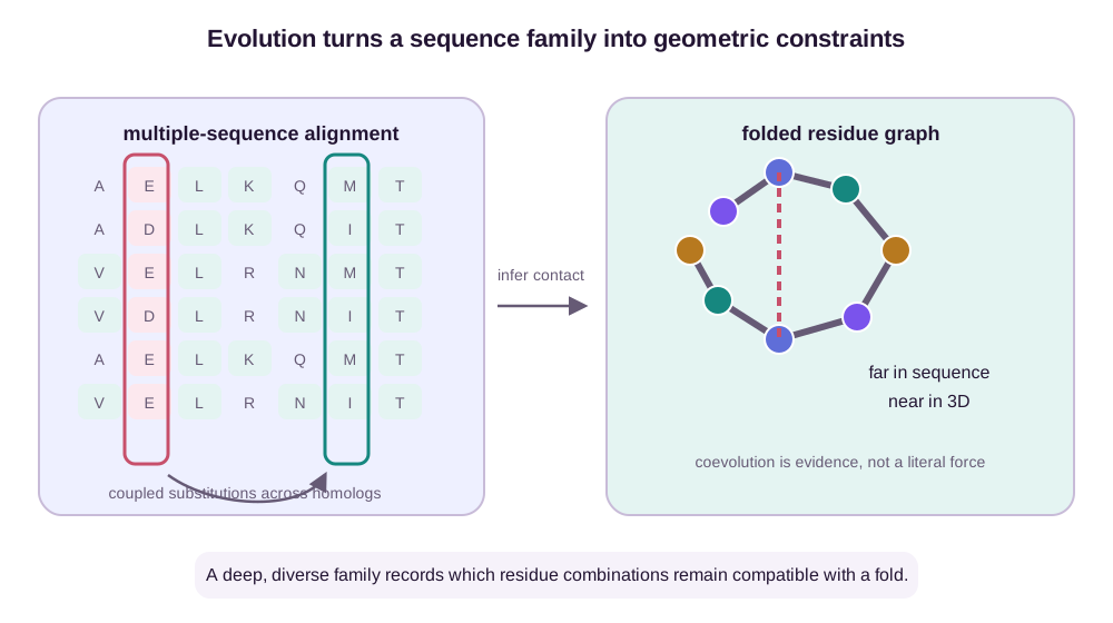
The caveat “rich sequence data” matters. A shallow MSA cannot reveal reliable covariance. A deep but redundant MSA can overstate one evolutionary branch. Homologs may share a fold while adopting different oligomeric states or functional conformations. Coevolution compresses family history into structural evidence, but it does not identify which experimental condition or dynamical state produced a particular structure.

Raw row count is therefore not effective depth. A common reweighting assigns sequence \(s\) weight \(w_s=1/n_s\), where \(n_s\) counts sequences above a chosen identity threshold around \(s\), and defines

\[N_{\mathrm{eff}}=\sum_s w_s.\]

If 80 of 100 rows form one near-identical clade, each receives weight \(1/80\) and the clade contributes only one effective sequence. If the remaining 20 rows are mutually distinct at the threshold, each contributes one, giving \(N_{\mathrm{eff}}=1+20=21\) rather than 100. The number 21 depends on the identity threshold and weighting rule; it is a diagnostic for redundancy, not a count of independent evolutionary experiments.

AlphaFold 1 Learned a Geometric Potential

AlphaFold 1 made an important shift from binary contact prediction to a distogram: for each residue pair \((i,j)\), the network predicted a categorical distribution over distance bins,

\[p_{ij}^{(b)} =P\!\left(d_{ij}\in[r_b,r_{b+1})\mid\text{sequence, MSA, templates}\right).\]

A contact map says only whether \(d_{ij}\) is below a threshold. A distogram distinguishes a tight contact from medium-range separation and represents uncertainty across several plausible distances. Pairwise features derived from the MSA and templates were processed by a deep residual network, producing distance and torsion distributions.

The predicted distributions did not directly place atoms. They became a learned potential, schematically

\[E(\mathbf{x}) =-\sum_{i<j}\log p_{ij}\!\left(d_{ij}(\mathbf{x})\right) +E_{\mathrm{torsion}}(\mathbf{x}) +E_{\mathrm{stereo}}(\mathbf{x}),\]

and coordinates were found by numerical optimization. The first term rewards structures whose pair distances fall in likely bins; torsional and stereochemical terms discourage locally impossible geometry and steric clashes. AlphaFold 1 therefore separated inference from realization: a neural network inferred geometric restraints, then a solver reconciled them in 3D. This neural-potential strategy was the core of the CASP13 system (Senior et al., 2020).

Three residues are enough to see what the solver contributes. Use distance bins short \((0,4)\) Å, medium \((4,8)\) Å, and long \((8,12)\) Å, with predicted probabilities

Pair	Short	Medium	Long
\((1,2)\)	0.80	0.15	0.05
\((2,3)\)	0.70	0.20	0.10
\((1,3)\)	0.10	0.20	0.70

Candidate \(A\) has distances \((d_{12},d_{23},d_{13})=(3,3,5)\) Å. Candidate \(B\) has \((5,5,9)\) Å. Both triples satisfy the triangle inequalities and can be realized by three points in space. Their pair-only energies are

\[E_A=-\log(0.80\times0.70\times0.20) =-\log(0.112)=2.189,\] \[E_B=-\log(0.15\times0.20\times0.70) =-\log(0.021)=3.863.\]

The pair potential prefers candidate \(A\) by \(1.674\) in these dimensionless log units. Torsion and stereochemical terms could reverse that ranking; this calculation isolates only the distogram contribution.

Taking the most likely bin independently gives the modal distances \((3,3,9)\) Å. They violate \(d_{13}\leq d_{12}+d_{23}\) because \(9>6\). Every pair marginal can look confident while their three modes describe no coordinate triangle. Candidate \(A\) compromises by placing pair \((1,3)\) in its lower-probability medium bin. Coordinate optimization is therefore not a cosmetic conversion from distances to atoms. It selects a jointly realizable configuration from pairwise beliefs that may be mutually inconsistent.

This division is interpretable but brittle. Pairwise distances need not be globally realizable. Torsion errors accumulate along a chain. Optimization can settle in a poor basin even when many individual restraints are correct. The central advance of AlphaFold 2 was to let coordinate construction participate in learned reasoning rather than appear only after it.

The Evoformer Makes Pair Geometry a Persistent State

AlphaFold 2 carries two main internal representations (Jumper et al., 2021):

• An MSA representation \(m_{si}\) stores features for sequence \(s\) at residue position \(i\).

• A pair representation \(z_{ij}\) stores the model’s evolving belief about the geometric relationship between residues \(i\) and \(j\).

The Evoformer alternates updates within and between these tracks. MSA attention asks which homologs and positions support a residue pattern. An outer-product mean transfers family-level correlations into pair space; schematically,

\[z_{ij} \leftarrow z_{ij} +\frac{1}{N_{\mathrm{seq}}} \sum_s \mathbf{a}(m_{si})\otimes\mathbf{b}(m_{sj}).\]

The outer product preserves interactions between channels at positions \(i\) and \(j\) rather than collapsing each column to a single covariance number. Learned projections then turn this family statistic into pair features.

Pair geometry must also be globally consistent. If residues \(i\) and \(j\) have a proposed relationship, every third residue \(k\) offers an indirect path \(i\rightarrow k\rightarrow j\) against which that proposal can be checked. A triangle multiplicative update has the schematic form

\[z_{ij} \leftarrow z_{ij} +\sum_k \mathbf{a}(z_{ik})\odot\mathbf{b}(z_{kj}),\]

with learned gates and projections omitted. Triangle attention performs a related comparison with data-dependent weights. The mechanism resembles geometric consistency: three edges form a triangle, so evidence on two sides constrains the third. It is learned algebra over pair features, not a hard Euclidean triangle solver, but the inductive bias is exactly the right one.

A scalar version exposes the arithmetic hidden by the channel notation. Take three MSA rows with projected values

\[\mathbf a_i=(1,0,2), \qquad \mathbf b_j=(2,1,1).\]

Their outer-product mean is just a mean of products,

\[\frac{1}{3}\sum_s a_{si}b_{sj} =\frac{2+0+2}{3}=\frac{4}{3}.\]

If the current scalar pair state is \(z_{ij}=0.20\) and a learned projection scales this statistic by \(0.5\), the update gives \(z_{ij}=0.20+0.5(4/3)=0.867\). The real module uses vectors, outer products, normalization, and learned gates, but its input remains an average of aligned cross-sequence evidence.

Now let two intermediate residues provide scalar pair paths

\[(z_{i1},z_{1j})=(0.4,0.5), \qquad (z_{i2},z_{2j})=(-0.2,0.3).\]

Their multiplicative evidence is \(0.4(0.5)+(-0.2)(0.3)=0.14\). With another scalar gate of \(0.5\), the pair state becomes \(0.867+0.070=0.937\). One path supports the relationship and one partially cancels it. A hard triangle rule would only accept or reject a metric triple; the learned update carries graded, channel-dependent evidence forward.

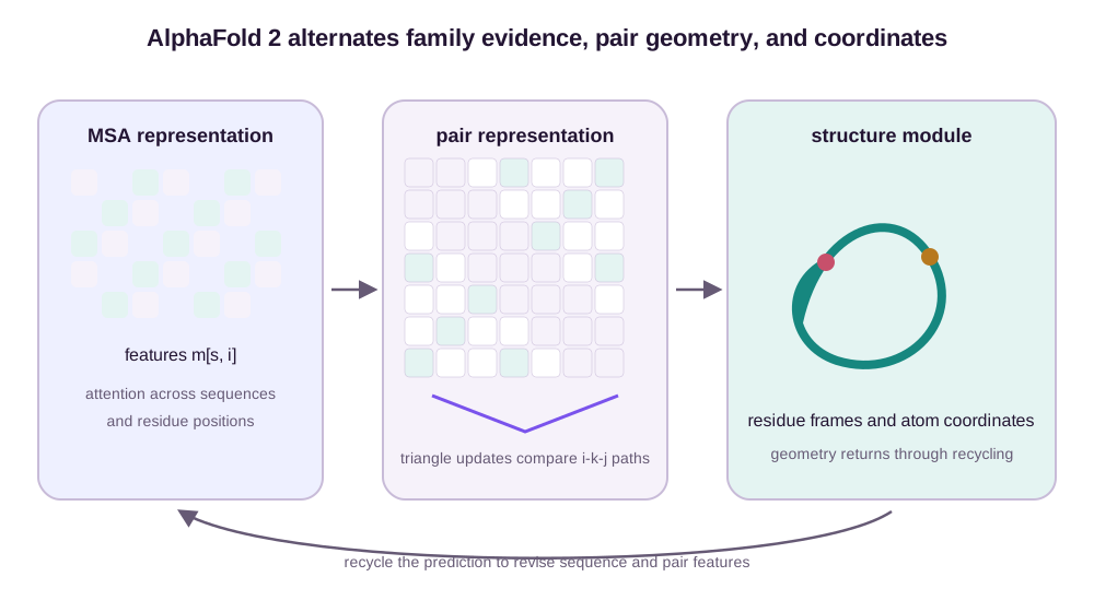
The pair representation is therefore more than a distance matrix. It becomes a workspace for orientation, compatibility, template evidence, and long-range constraint propagation. This is why reducing AlphaFold 2 to “a Transformer on an MSA” misses the architectural point: the model devotes comparable effort to reasoning in the complete graph of residue pairs.

That complete graph sets the computational scale. With \(N_{\mathrm{seq}}\) MSA rows, length \(L\), MSA width \(c_m\), and pair width \(c_z\), the two persistent tensors require

\[O(N_{\mathrm{seq}}Lc_m) \qquad\text{and}\qquad O(L^2c_z)\]

memory. For \(N_{\mathrm{seq}}=512\), \(L=1000\), \(c_m=256\), and 32-bit values, the MSA tensor alone occupies about 524 MB. A pair tensor with \(c_z=128\) occupies another 512 MB, before storing attention intermediates, gradients, or recycled copies.

A direct triangle update visits triples \((i,k,j)\) and scales as \(O(L^3c_z)\) after channel projections. At \(L=1000\) and \(c_z=128\), that count is about \(1.28\times10^{11}\) scalar path-channel contributions per block. Kernels, chunking, reduced precision, and parallel hardware change runtime and peak memory, but not the leading length dependence. Doubling \(L\) multiplies pair memory by four and naive triangle work by eight. Cropping and memory-efficient implementations are responses to this pair geometry, not incidental engineering details.

Local Frames Turn Pair Reasoning Into Equivariant Coordinates

The AlphaFold 2 structure module represents each residue backbone as a rigid frame

\[T_i=(R_i,\mathbf{t}_i),\]

where \(R_i\in SO(3)\) is an orientation and \(\mathbf{t}_i\in\mathbb{R}^3\) is a translation. Side-chain torsions place atoms relative to that frame. The model iteratively updates these frames using single-residue and pair features.

Invariant point attention attaches learned query and key points to local frames. A query point \(\mathbf{q}_{ih}\) in residue \(i\)’s local coordinates becomes \(R_i\mathbf{q}_{ih}+\mathbf{t}_i\) globally; a key point on residue \(j\) is transformed similarly. Their squared distance,

\[\left\| R_i\mathbf{q}_{ih}+\mathbf{t}_i -R_j\mathbf{k}_{jh}-\mathbf{t}_j \right\|^2,\]

is unchanged if the whole protein is rotated and translated. Attention can therefore depend on 3D geometry without choosing a privileged laboratory frame. When the input frames undergo a global rigid transformation, the output frames and atoms transform with them: the coordinate construction is equivariant.

A numerical check makes the cancellation concrete. Let residue \(i\) have frame \(R_i=I\) and \(\mathbf{t}_i=(1,0,0)\), with local query point \(\mathbf{q}=(1,0,0)\). Its global position is \((2,0,0)\). Let residue \(j\) have a \(90^\circ\) rotation about \(z\), translation \((0,2,0)\), and local key point \((1,0,0)\). Its global position is \((0,3,0)\), so the squared query–key distance is \(2^2+(-3)^2=13\). Now rotate the entire complex by another \(90^\circ\) about \(z\) and translate it by \((5,-1,2)\). The two points become \((5,1,2)\) and \((2,-1,2)\); their squared distance is again \(3^2+2^2=13\). Algebraically, each frame changes as

\[R_i' = S R_i, \qquad \mathbf{t}_i'=S\mathbf{t}_i+\mathbf{u},\]

so every transformed point is \(S(R_i\mathbf{q}+\mathbf{t}_i)+\mathbf{u}\). Translation disappears from a difference, and orthogonality gives \(\|S\mathbf{v}\|^2=\|\mathbf{v}\|^2\). This is an identity of the representation, not a pattern that must be learned from rotated examples. The broader group-theoretic statement is developed in the symmetry and equivariance chapter; here, the important point is that the identity is built into the coordinate interface.

The training loss uses the same local-frame logic. Frame-aligned point error compares a predicted atom \(\widehat{\mathbf{x}}_j\) and true atom \(\mathbf{x}_j\) as seen from residue \(i\):

\[\operatorname{FAPE}_{ij} =\left\| \widehat{T}_i^{-1}\widehat{\mathbf{x}}_j -T_i^{-1}\mathbf{x}_j \right\|.\]

A global rotation or translation cancels inside both inverse frames. The loss rewards correct relative geometry and does not require a separate global alignment. Because every residue provides a local viewpoint, it strongly constrains both local side-chain packing and long-range placement.

FAPE is invariant, but it is not blind. Suppose the true residue frame is \((I,(1,0,0))\) and the true atom is \((2,2,0)\). The atom has true local coordinates \((1,2,0)\). Take a predicted frame with a \(90^\circ\) rotation about \(z\) and translation \((0,1,0)\), and a predicted atom at \((-2.5,2,0)\). Applying the predicted inverse frame gives \((1,2.5,0)\), hence \(\operatorname{FAPE}=0.5\) Å. If both structures are jointly rotated and translated, both inverse-frame coordinates remain \((1,2,0)\) and \((1,2.5,0)\). The loss stays at \(0.5\) Å. It ignores only the arbitrary global pose; an incorrect local relationship still incurs error.

Recycling closes the loop. Predicted coordinates are converted back into pair and single features, then passed through the network again. The model can revise an MSA-derived hypothesis after seeing the geometry it produced. AlphaFold 2 is thus not a one-pass decoder: it alternates constraint inference and coordinate realization inside the learned system.

Confidence Is Part of the Prediction

A single coordinate file can look authoritative even where the model has little evidence. AlphaFold counters this with confidence estimates at different scales.

pLDDT is a per-residue prediction of local structural accuracy. High pLDDT supports interpreting the local backbone and, at the highest values, often side-chain placement. Low pLDDT is deliberately ambiguous: it may indicate insufficient evolutionary information, an intrinsically disordered region, a flexible linker, an unusual state, or ordinary model error. Applying AlphaFold 2 across the human proteome demonstrated that pLDDT was calibrated against held-out experimental structures and made residue-level confidence essential to large-scale use (Tunyasuvunakool et al., 2021).

Predicted aligned error (PAE) is pairwise. PAE\((i,j)\) estimates the position error at residue \(i\) when prediction and reference are aligned on residue \(j\). A two-domain protein can have high pLDDT within both domains but high cross-domain PAE: each domain is locally convincing, while their relative orientation is not. Collapsing these signals into one global score discards the distinction a structural biologist needs.

Consider four residues split into two rigid domains, \(A=\{1,2\}\) and \(B=\{3,4\}\). Suppose their pLDDT values are \((92,90,91,89)\), with mean \(90.5\), while the predicted aligned-error matrix in Å is

\[\operatorname{PAE}= \begin{pmatrix} 1&2&18&20\\ 2&1&17&19\\ 19&18&1&2\\ 20&19&2&1 \end{pmatrix}.\]

The diagonal blocks support both local folds. The large off-diagonal blocks say that aligning on one domain leaves the other poorly placed. Thus the defensible decision is to use each domain as a local structural hypothesis while declining to treat their relative orientation as a resolved interface. High local confidence and high cross-domain uncertainty are not contradictory; they concern different random variables, alignments, and spatial granularities.

That distinction matters when interpreting the numbers. pLDDT predicts an expected local lDDT-like accuracy for each residue without requiring a single global superposition. PAE\((i,j)\) predicts the error at \(i\) after an alignment centered on \(j\) and is therefore pairwise and, in general, directional. Both are learned estimates calibrated empirically against held-out structures from a reference population. Calibration means that bins of predictions have matched frequencies on that evaluation population; it does not turn either score into a posterior guarantee for a novel chemistry, conformational state, or interaction context.

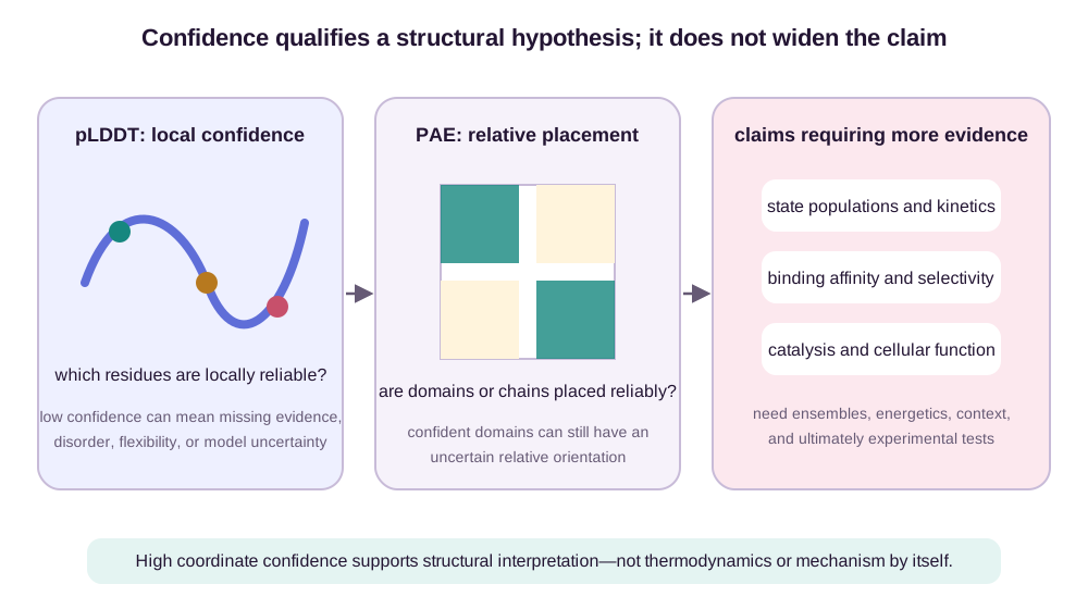
Confidence is model- and task-specific. A high score means the model expects its coordinates to resemble a relevant experimental structure under its training distribution. It is not a posterior probability that the protein always adopts this conformation, nor a certificate that an interface forms in the cell.

AlphaFold 3 Generalizes the Coordinate Space

AlphaFold 2’s residue frames and torsion hierarchy are elegant for proteins, but less natural for a complex containing RNA bases, a metal ion, a covalently modified residue, and a flexible small molecule. AlphaFold 3 changes the output representation: its diffusion module operates on raw atom coordinates for a heterogeneous complex (Abramson et al., 2024).

The trunk still builds single-token and token-pair representations. Polymer residues and ligand atoms or groups become tokens; atom-level features retain the fine chemical detail. A simplified Pairformer performs pair and single updates while omitting the persistent MSA track of the AlphaFold 2 Evoformer. The resulting conditioning is passed to an all-atom denoiser.

For a clean complex with coordinates \(\mathbf{x}_0\), diffusion training constructs noisy coordinates

\[\mathbf{x}_\sigma =\mathbf{x}_0+\sigma\boldsymbol{\epsilon}, \qquad \boldsymbol{\epsilon}\sim\mathcal{N}(\mathbf{0},\mathbf{I}),\]

after randomizing global rotation and translation. The network predicts a less noisy structure conditioned on sequence, chemistry, MSA-derived information, templates, and pair features. Sampling starts from coordinate noise and repeatedly denoises toward a joint complex.

The corruption itself respects rigid motion. Take two clean atoms at \((0,0,0)\) and \((2,0,0)\), noise vectors \((1,0,0)\) and \((0,1,0)\), and \(\sigma=0.5\). Their noisy coordinates are \((0.5,0,0)\) and \((2,0.5,0)\). Rotate by \(90^\circ\) about \(z\) and translate by \((3,-1,0)\). If the noise vectors rotate with the atoms, corruption gives \((3,-0.5,0)\) and \((2.5,1,0)\)—exactly the rigid transform of the original noisy pair. Because isotropic Gaussian noise has the same distribution after rotation, this equality also holds in distribution when fresh noise is drawn. It is the data-generating process, not yet a guarantee about the learned denoiser.

Unlike the frame-based AlphaFold 2 structure module, the published AlphaFold 3 diffusion module does not use rotational frames or explicitly equivariant processing. Random rigid augmentation teaches the desired behavior statistically. This simplifies the decoder and avoids hand-designing a coordinate hierarchy for every molecular type, but it exchanges exact architectural symmetry for learned symmetry and extensive augmentation.

The distinction can be tested directly: corrupt a complex, transform both clean and noisy coordinates, and compare the transformed denoising prediction with the prediction obtained from the transformed input. Equality of the corruption law is an identity; equality of these two network outputs is an empirical augmentation check and may be approximate. The diffusion and flow-matching chapter develops the reverse-time mechanics. Here the relevant modeling choice is narrower: atom-space diffusion gives one decoder a common coordinate language for proteins, nucleic acids, ions, and ligands.

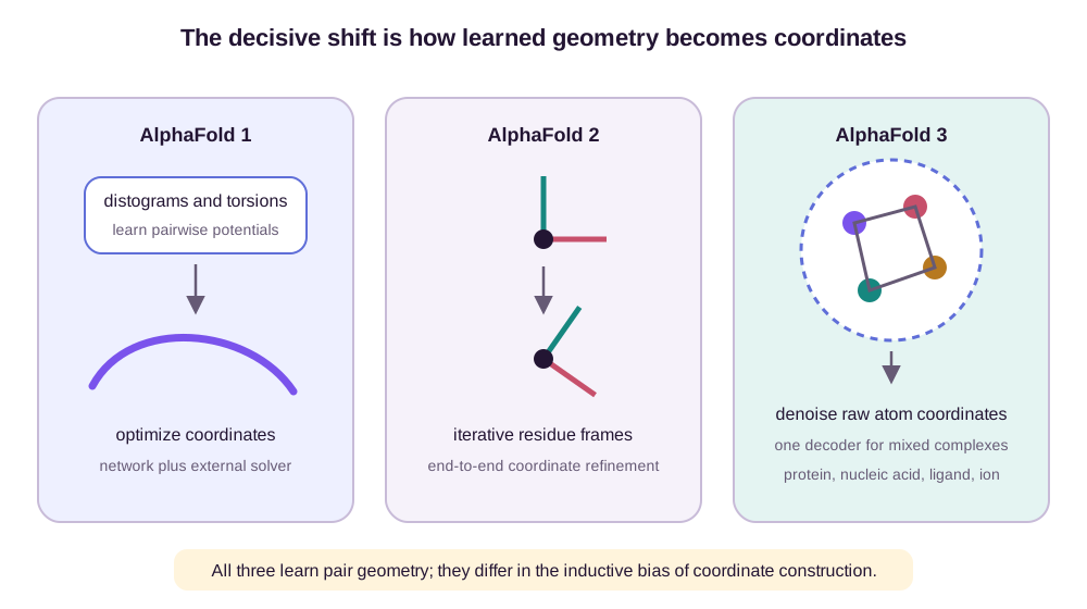
Diffusion also changes the interpretation of multiple outputs. Stochastic sampling can expose alternative coordinate hypotheses and uncertainty. It does not automatically produce a thermodynamic ensemble. A Boltzmann ensemble requires correct relative state probabilities under specified conditions; a kinetic model requires transition rates or time-resolved dynamics. A denoiser trained to reproduce deposited structures is optimized for structural accuracy, not those quantities.

For example, imagine that 100 sampling runs yield pose A 70 times and pose B 30 times. If those were independent equilibrium samples at \(298\) K, then with \(RT\approx0.592\) kcal/mol the ratio would imply

\[G_B-G_A=RT\log\frac{70}{30}\approx0.50\ \text{kcal/mol}.\]

But AlphaFold sampling frequencies also reflect training-set prevalence, conditioning, initialization, diffusion schedule, and sampling implementation. They are not labeled with temperature or a physical measure. The 70:30 split supports the operational statement that both hypotheses are reachable and A is more frequently returned by this procedure. It does not support the thermodynamic equation above.

What a Predicted Structure Does—and Does Not—Establish

A confident structure is a powerful hypothesis. It can suggest domain boundaries, catalytic residues, mutation sites, binding pockets, and plausible interfaces. AlphaFold 3 extends this reach by predicting joint complexes, where ligand and partner geometry can be reasoned about together. But coordinates alone do not close the causal chain from sequence to function.

Dynamics and state populations

Proteins fluctuate within basins and transition between conformations. Transporters alternate inward- and outward-facing states; kinases switch regulatory conformations; disordered regions may never adopt one dominant fold. A default AlphaFold 2 run typically concentrates on one structurally plausible state. MSA subsampling can encourage alternative conformations for some transporters and receptors, as demonstrated experimentally in a targeted protocol (del Alamo et al., 2022). Those samples are useful hypotheses, but their frequency is not an equilibrium population, and model iteration is not physical time.

Binding geometry and affinity

A predicted complex can answer “how might these molecules fit?” It does not by itself answer “how tightly do they bind?” Binding free energy includes solvent reorganization, entropy, protonation, competing states, and concentration conventions. The thermodynamic relation

\[\Delta G^\circ = RT\log\frac{K_d}{C^\circ}, \qquad C^\circ=1\ \mathrm{M},\]

contains information absent from one pose. A geometrically credible protein–ligand complex can still have weak affinity, and a wrong protonation state can reverse an interaction. Pose confidence should guide docking analysis and experiments, not substitute for affinity measurement.

The logarithm makes a modest energetic omission consequential. At \(298\) K, two ligands with nearly indistinguishable predicted poses but binding free energies of \(-8\) and \(-6\) kcal/mol have

\[K_{d,A}\approx1.35\ \mu\mathrm{M}, \qquad K_{d,B}\approx39.7\ \mu\mathrm{M}.\]

A \(2\) kcal/mol difference therefore corresponds to roughly a \(29\)-fold affinity ratio. Solvent displacement, conformational entropy, protonation, and competing solution states can easily contribute at that scale while leaving the static bound geometry visually similar.

Structure and function

Structural similarity supports functional hypotheses, but identical folds can support different substrates, regulation, or cellular roles. Catalysis depends on electronic structure and transition states, not just the ground-state arrangement of heavy atoms. Function also depends on expression, localization, partners, modifications, and environmental conditions. A predicted active-site geometry is a reason to run a biochemical assay; it is not the assay result.

These limitations do not diminish structure prediction. They locate it correctly. AlphaFold transformed a scarce experimental input into an abundant computational hypothesis, and confidence scores make those hypotheses unusually actionable. The next scientific step is chosen by the claim: molecular dynamics or ensemble models for conformational populations, free-energy methods and assays for binding, mutagenesis and cellular experiments for mechanism and function.

The practical contract is therefore explicit. Coordinates plus local confidence support a claim about a structural hypothesis under the supplied sequence, chemical context, and model distribution. Low PAE can additionally support relative placement at the indicated residue, domain, or chain granularity. Neither output alone identifies an equilibrium population or transition rate; that requires a defined physical ensemble and dynamical evidence. Neither establishes affinity; that requires a free-energy calculation with stated conditions or a binding assay. Neither establishes molecular or cellular function; that requires a mechanistic prediction linked to perturbation and experiment. These are different target variables, not progressively stricter confidence thresholds on the same variable.

The Representation Is the Breakthrough

The durable lesson across AlphaFold 1–3 is not that one neural architecture replaced another. Each generation chose a better intermediate object for the uncertainty it had to resolve.

AlphaFold 1 learned distributions over pair geometry rather than forcing an early coordinate guess. AlphaFold 2 made the pair representation a persistent reasoning space and let local frames connect that space to equivariant coordinates. AlphaFold 3 kept learned pair constraints but broadened the coordinate language to all atoms in mixed biomolecular complexes through diffusion.

MSAs, pair matrices, residue frames, and noisy atom clouds are not interchangeable encodings. Each exposes some constraints and hides others. Their success comes from matching representation to inference: evolution constrains residue compatibility, triangles constrain global geometry, frames remove arbitrary global pose, and diffusion accommodates heterogeneous chemistry. Confidence then marks where the inferred structure is stable enough to use—and where biological interpretation must wait for more evidence.

The information flow can be read as a sequence of contracts rather than a stack of opaque modules. An MSA row is an observed sequence, while an MSA embedding is a learned summary; neither is a direct-contact map. A pair state is indexed by residue or token pairs, but its channels are learned latent variables rather than calibrated distances unless a supervised head gives them that meaning. A residue frame or atom cloud is a geometric realization of those constraints, and its equivariance or augmentation behavior says how it changes under coordinates—not whether the biology is correct. Finally, pLDDT and PAE attach predicted error variables to that realization. Keeping those types separate prevents a common interpretive slide from “the model represented a dependency” to “the model established a mechanism.”

Object	Exact or learned property used downstream	Claim it can support	Information still missing
Weighted MSA	Sequence identities and redundancy weights are observed; embeddings are learned	Evolutionary compatibility under the sampled family	Direct versus indirect cause, assay conditions
Pair representation	Persistent \(L\times L\) or token-pair indexing; channel semantics are learned	A globally revised hypothesis about pair geometry	A guaranteed realizable metric or unique structure
Residue frames	Rigid transformations obey exact composition rules	Protein coordinates independent of laboratory pose	Population weights and kinetic rates
Atom diffusion samples	Corruption law is rotation-invariant; denoising symmetry is learned approximately	One or more joint-complex structural hypotheses	Boltzmann weights, affinity, chemical mechanism
pLDDT and PAE	Learned, calibrated error summaries with distinct alignment conventions	Local accuracy and relative-placement decisions at stated granularity	Out-of-distribution guarantees or biological truth

This view also clarifies why AlphaFold 3 is both a continuation and a genuine change. It retains a pairwise constraint state because chemistry still has long-range consistency, but replaces a protein-specific coordinate contract with a heterogeneous atom-space one. That broader output space makes interaction prediction possible within one model; it also raises the cost of treating a coordinate sample as a complete explanation. The model can place an ion, ligand, DNA base, and protein side chain together without thereby assigning the correct protonation ensemble, concentration dependence, or catalytic rate.

For downstream work, the most useful question is therefore not whether a structure is “confident” in the abstract. It is which output variable bears on the proposed decision. A mutation near a high-pLDDT pocket may be a sensible experiment even when two domains have uncertain relative orientation. An interface claim needs low cross-chain PAE or an interaction-specific confidence signal, not merely excellent monomer pLDDT. An affinity claim needs thermodynamics, and a functional claim needs perturbation. AlphaFold’s representational breakthrough matters precisely because it makes the structural portion of that chain much more reliable while leaving the remaining links visible.

---

References

Marks, D. S., Colwell, L. J., Sheridan, R., Hopf, T. A., Pagnani, A., Zecchina, R., & Sander, C. (2011). Protein 3D Structure Computed from Evolutionary Sequence Variation. PLOS ONE, 6(12), e28766. ↩

Senior, A. W., Evans, R., Jumper, J., et al. (2020). Improved Protein Structure Prediction Using Potentials from Deep Learning. Nature, 577, 706–710. ↩

Jumper, J., Evans, R., Pritzel, A., et al. (2021). Highly Accurate Protein Structure Prediction with AlphaFold. Nature, 596, 583–589. ↩

Tunyasuvunakool, K., Adler, J., Wu, Z., et al. (2021). Highly Accurate Protein Structure Prediction for the Human Proteome. Nature, 596, 590–596. ↩

Abramson, J., Adler, J., Dunger, J., et al. (2024). Accurate Structure Prediction of Biomolecular Interactions with AlphaFold 3. Nature, 630, 493–500. ↩

del Alamo, D., Sala, D., Mchaourab, H. S., & Meiler, J. (2022). Sampling Alternative Conformational States of Transporters and Receptors with AlphaFold2. eLife, 11, e75751. ↩