Discrete Flow and Generator Matching

Adapted from my 2025 Machine Learning for Molecules and Geometric Deep Learning lectures. Here generation is governed by continuous-time Markov rates that determine waiting times as well as destinations; see ODEs, SDEs, and Probability Flow for the continuous counterpart and Generative Flow Networks for flow balance on construction graphs.

A continuous flow moves a point by an infinitesimal vector. That picture breaks on a categorical state space. There is no state halfway between carbon and nitrogen, no amino acid infinitesimally close to glycine, and no fractional bond order hiding between two graph categories.

Probability can nevertheless evolve continuously in time. The state remains discrete, but the chance of jumping changes smoothly. A continuous-time Markov chain replaces velocity by a collection of transition rates. Its master equation replaces the continuity equation. Once that replacement is made, much of flow matching survives: choose a tractable path of probability distributions, construct simple dynamics conditioned on a data endpoint, and regress their posterior average.

The generator is the object that makes this analogy precise. On a finite state space it is a rate matrix. On Euclidean or geometric spaces it becomes a differential operator. Generator matching therefore does more than rename discrete flow matching. It isolates the common infinitesimal structure behind ODEs, diffusions, jumps, and mixtures of them.

A rate is an infinitesimal probability of jumping

Let \(\mathcal{S}\) be a finite state space and let \(X_t\in\mathcal{S}\). For two distinct states \(x,y\in\mathcal{S}\), define the time-dependent jump rate

\[q_t(y\mid x)\geq 0, \qquad y\neq x.\]

Our notation places the destination first: \(q_t(y\mid x)\) is the rate of jumping from \(x\) to \(y\). Over a short interval of length \(h>0\),

\[\Pr(X_{t+h}=y\mid X_t=x) =h q_t(y\mid x)+o(h), \qquad y\neq x.\]

The total exit rate from \(x\) is

\[\lambda_t(x)=\sum_{y\neq x}q_t(y\mid x).\]

Consequently, the probability of staying at \(x\) is

\[\Pr(X_{t+h}=x\mid X_t=x) =1-h\lambda_t(x)+o(h).\]

It is convenient to define the diagonal entry as

\[q_t(x\mid x)=-\lambda_t(x).\]

The matrix \(Q_t\) with entries \((Q_t)_{yx}=q_t(y\mid x)\) then has nonnegative off-diagonal entries and columns that sum to zero. Some references put sources in rows and write \(p_tQ_t\) instead. Nothing substantive changes, but mixing the two conventions silently transposes every equation.

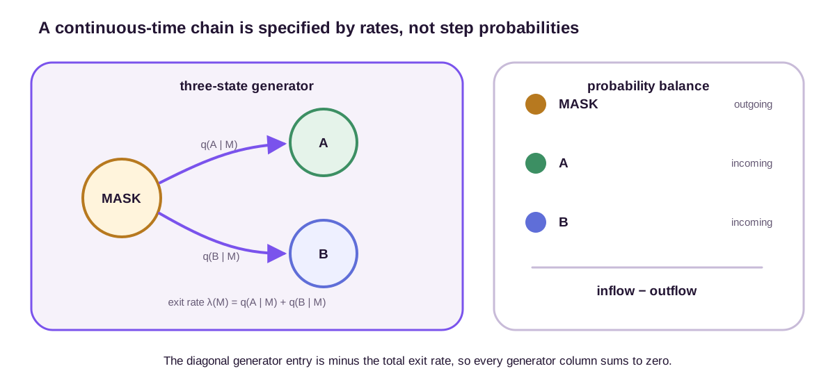
Let \(p_t(x)=\Pr(X_t=x)\) and regard \(p_t\) as a column vector. Probability obeys the master equation, also called the Kolmogorov forward equation:

\[\frac{d}{dt}p_t(y) =\sum_{x\in\mathcal{S}}q_t(y\mid x)p_t(x).\]

Separating the diagonal term exposes the probability balance:

\[\frac{d}{dt}p_t(y) =\underbrace{\sum_{x\neq y}q_t(y\mid x)p_t(x)}_{\text{inflow}} -\underbrace{\lambda_t(y)p_t(y)}_{\text{outflow}}.\]

In matrix notation, \(\dot p_t=Q_t p_t\). This is the discrete analogue of a continuity equation. A continuous velocity transports density through spatial flux; a generator transports probability through jumps between named states.

The convention becomes concrete in the mask example used throughout this post. Order the states as \((M,A,B)\) and suppose a masked token leaves at total rate \(r_t\), choosing \(A\) with probability \(0.6\) and \(B\) with probability \(0.4\). Then

\[Q_t= \begin{pmatrix} -r_t & 0 & 0\\ 0.6r_t & 0 & 0\\ 0.4r_t & 0 & 0 \end{pmatrix}.\]

This small matrix is an executable test of every sign. Its off-diagonal entries are nonnegative. Each column sums to zero, or \(\mathbf{1}^{\mathsf T}Q_t=0\), so

\[\frac{d}{dt}\mathbf{1}^{\mathsf T}p_t =\mathbf{1}^{\mathsf T}Q_tp_t=0.\]

Thus the master equation conserves total probability. Over a short interval,

\[P_{t,t+h}=I+hQ_t+O(h^2).\]

For the linear schedule considered below, \(r_{0.5}=2\). Freezing the rates for \(h=0.1\) gives

\[I+hQ_{0.5} = \begin{pmatrix} 0.8&0&0\\ 0.12&1&0\\ 0.08&0&1 \end{pmatrix}.\]

Its columns sum to one and all entries are nonnegative. Acting on \(p_{0.5}=(0.5,0.3,0.2)^{\mathsf T}\) produces \((0.4,0.36,0.24)^{\mathsf T}\). The approximation becomes an exact transition matrix \(e^{hQ}\) when \(Q\) is time-homogeneous; \(I+hQ_t\) is only a first-order numerical choice.

That distinction sets a hard boundary. The frozen-rate step has stay probability \(1-h\lambda_t(x)\), so it is a probability kernel only if \(h\lambda_t(x)\leq 1\). At \(t=0.9\) the linear mask schedule has \(r_t=10\). A step of \(h=0.2\) would assign the mask a stay probability \(-1\). This is not merely inaccurate—it is not a probability distribution at all. Nonnegative learned rates guarantee an infinitesimal generator; they do not make an arbitrarily large Euler step valid.

The generator describes what every observable does next

A rate matrix is useful on a finite set, but the more durable definition acts on test functions. For any observable \(f:\mathcal{S}\to\mathbb{R}\), define

\[(\mathcal{L}_t f)(x) =\lim_{h\downarrow 0} \frac{\mathbb{E}[f(X_{t+h})\mid X_t=x]-f(x)}{h}.\]

Substituting the short-time transition law gives

\[(\mathcal{L}_t f)(x) =\sum_{y\neq x}q_t(y\mid x)\bigl[f(y)-f(x)\bigr].\]

The generator answers a local question: if the process is currently at \(x\), how quickly will the expected value of any observable change? The master equation is its dual statement about probability. With

\[\langle p,f\rangle =\sum_{x\in\mathcal{S}}p(x)f(x),\]

the weak forward equation is

\[\frac{d}{dt}\langle p_t,f\rangle =\langle p_t,\mathcal{L}_t f\rangle.\]

Writing \(\mathcal{L}_t^*\) for the adjoint yields \(\partial_t p_t=\mathcal{L}_t^*p_t\). On a finite state space, this is exactly \(\dot p_t=Q_tp_t\). For an ODE, the generator is \(\mathcal{L}_t f=\nabla f^{\mathsf T}v_t\). For a diffusion, it adds a Hessian term. For a jump process, it sums or integrates finite differences. Generator matching begins from this operator-level identity (Holderrieth et al., 2025).

With the column convention above, the two matrix actions are worth separating:

\[\dot p_t=Q_tp_t, \qquad \mathcal{L}_tf=Q_t^{\mathsf T}f.\]

The transpose is not a second modeling choice. It is forced by duality:

\[\frac{d}{dt}(f^{\mathsf T}p_t) =f^{\mathsf T}Q_tp_t =(Q_t^{\mathsf T}f)^{\mathsf T}p_t.\]

For a numerical check, assign values \(f(M)=0\), \(f(A)=1\), and \(f(B)=3\). At \(t=0.5\), the mask’s instantaneous observable drift is

\[(\mathcal{L}_{0.5}f)(M) =1.2(1-0)+0.8(3-0)=3.6,\]

while it is zero at the two absorbing tokens. Since half of the marginal mass is masked,

\[\langle p_{0.5},\mathcal{L}_{0.5}f\rangle =0.5\times 3.6=1.8.\]

The designed marginal path below has

\[\mathbb{E}[f(X_t)] =0.6t\times 1+0.4t\times 3=1.8t,\]

whose derivative is also \(1.8\). This agreement is a compact orientation test: if either the source/destination indices or the transpose were reversed, the equality would fail.

A mask-to-token chain is a complete worked example

Consider the three-state space

\[\mathcal{S}=\{M,A,B\},\]

where \(M\) is a mask token. Let the data endpoint \(Z\) equal \(A\) with probability \(0.6\) and \(B\) with probability \(0.4\). We want a path that begins fully masked and ends at this data distribution. Choose an increasing schedule \(\kappa_t\) satisfying \(\kappa_0=0\) and \(\kappa_1=1\), and define the endpoint-conditioned path

\[p_t(x\mid Z=z) =(1-\kappa_t)\,\delta_M(x) +\kappa_t\,\delta_z(x).\]

Conditioned on \(z\), a chain realizes this path by jumping from \(M\) to \(z\) at rate

\[r_t=\frac{\dot\kappa_t}{1-\kappa_t},\]

with \(z\) absorbing. To verify the construction, let \(s_t\) be the conditional probability of still being masked. The master equation gives

\[\dot s_t=-r_ts_t.\]

Since \(s_t=1-\kappa_t\),

\[-r_ts_t =-\frac{\dot\kappa_t}{1-\kappa_t}(1-\kappa_t) =-\dot\kappa_t,\]

which is exactly \(d(1-\kappa_t)/dt\).

The same calculation determines the event time, not just the marginal. If \(T\) is the unmasking time, its conditional survival probability is

\[S(t)=\Pr(T>t) =\exp\!\left(-\int_0^t r_s\,ds\right) =1-\kappa_t.\]

The integrated hazard is therefore

\[H(t)=\int_0^t r_s\,ds=-\log(1-\kappa_t),\]

and the jump-time density is

\[f_T(t)=r_tS(t)=\dot\kappa_t.\]

For the linear schedule \(\kappa_t=t\), \(T\) is uniform on \([0,1]\) even though the instantaneous rate \(1/(1-t)\) diverges. One exact inverse sample is obtained by drawing \(U\sim\operatorname{Uniform}(0,1)\) and setting \(T=\kappa^{-1}(U)\). Equivalently, draw an exponential threshold \(E=-\log U\) and solve \(H(T)=E\); for the linear path this gives \(T=1-U\), which has the same uniform law. If the survival draw happens to be \(U=0.25\), the jump occurs at \(T=0.75\). Its destination is then \(A\) with probability \(0.6\) and \(B\) with probability \(0.4\). Thus this process has exactly one event, and its event time can be sampled without stepping through the singular endpoint.

Marginalizing over \(Z\) gives

\[p_t(M)=1-\kappa_t, \qquad p_t(A)=0.6\kappa_t, \qquad p_t(B)=0.4\kappa_t.\]

While the current state is \(M\), its endpoint remains hidden. The marginal chain averages the two conditional possibilities:

\[q_t(A\mid M)=0.6r_t, \qquad q_t(B\mid M)=0.4r_t.\]

Take the linear schedule \(\kappa_t=t\). At \(t=0.5\), \(r_t=2\) and the current marginal is

\[p_{0.5}=(0.5,0.3,0.2)^{\mathsf T}\]

in the order \((M,A,B)\). A forward Euler step of size \(h=0.1\) gives

\[p_{0.6} \approx p_{0.5}+h\dot p_{0.5} =(0.5,0.3,0.2)^{\mathsf T} +0.1(-1,0.6,0.4)^{\mathsf T} =(0.4,0.36,0.24)^{\mathsf T}.\]

This matches the designed path at \(\kappa_{0.6}=0.6\). The example also exposes a numerical issue: \(r_t=1/(1-t)\) diverges near the endpoint. The integrated hazard is correct—the surviving masked mass shrinks exactly like \(1-t\)—but a fixed-step sampler must shorten its step or force the final unmasking.

There is no contradiction between the finite event law and the divergent rate. The rate is conditioned on the increasingly rare event that the token is still masked. The expected marginal exit flux is

\[p_t(M)r_t=(1-t)\frac{1}{1-t}=1,\]

which stays finite. This distinction between a conditional hazard and a marginal flux will matter again when comparing event-driven and batched simulation.

Conditional paths make an intractable marginal generator learnable

The toy calculation scales because it has a general form. Draw a target endpoint \(Z\sim p_{\mathrm{data}}\) and choose tractable conditional paths \(p_t(x\mid z)\). Their mixture defines the desired marginal path:

\[p_t(x) =\sum_z p_{\mathrm{data}}(z)p_t(x\mid z).\]

Suppose \(q_t^z(y\mid x)\) generates the conditional path for endpoint \(z\). Then the marginal rate is the posterior average

\[q_t(y\mid x) =\sum_z q_t^z(y\mid x)p_t(z\mid x) =\mathbb{E}\!\left[q_t^Z(y\mid x)\mid X_t=x\right].\]

The identity follows directly from the master equation:

\[\begin{aligned} \dot p_t(y) &=\sum_z p_{\mathrm{data}}(z) \sum_x q_t^z(y\mid x)p_t(x\mid z)\\ &=\sum_x p_t(x) \sum_z q_t^z(y\mid x)p_t(z\mid x). \end{aligned}\]

The posterior \(p_t(z\mid x)\) is usually intractable, which is exactly why the marginal rates cannot be written down. Training avoids evaluating it. We sample \(Z\) from data, sample \(X_t\) from the tractable conditional path, and regress the known conditional rate target.

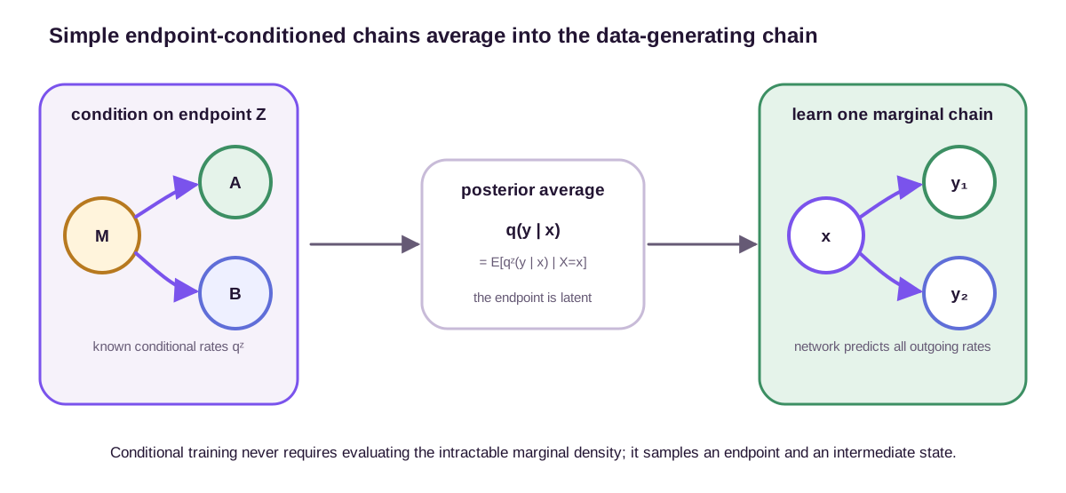
Let \(q_\theta(\cdot\mid x,t)\) denote the network’s vector of outgoing rates. With a Bregman divergence \(D\), the conditional discrete flow-matching objective has the form

\[\mathcal{J}_{\mathrm{CDFM}}(\theta) =\mathbb{E}_{t,Z,X_t} \left[ D\!\left(q_t^Z(\cdot\mid X_t), q_\theta(\cdot\mid X_t,t)\right) \right].\]

The mean claim is easiest to see before invoking a general divergence. At \(t=0.5\) and \(X_t=M\), the conditional outgoing-rate target on coordinates \((A,B)\) is

\[Y= \begin{cases} (2,0), & Z=A,\\ (0,2), & Z=B. \end{cases}\]

The posterior over endpoints is still \((0.6,0.4)\) because observing the common mask reveals no endpoint information. For a prediction \((a,b)\), the conditional squared risk is

\[R(a,b) =0.6\bigl[(a-2)^2+b^2\bigr] +0.4\bigl[a^2+(b-2)^2\bigr].\]

Setting its two derivatives to zero gives \((a,b)=(1.2,0.8)\), exactly the marginal rates used in the explicit matrix. In general, if \(W=(X_t,t)\), \(Y=q_t^Z(\cdot\mid X_t)\), and \(\mu(W)=\mathbb{E}[Y\mid W]\), then

\[\mathbb{E}\|g(W)-Y\|^2 =\mathbb{E}\|g(W)-\mu(W)\|^2 +\mathbb{E}\|Y-\mu(W)\|^2.\]

The cross term vanishes after conditioning on \(W\). The second term does not depend on \(g\), so the population minimizer is the marginal generator.

The same arithmetic conditional mean minimizes a Bregman loss generated by a twice-differentiable, strictly convex \(\phi\) when its orientation is

\[D_\phi(y,g) =\phi(y)-\phi(g)-\nabla\phi(g)^{\mathsf T}(y-g),\]

with the target in the first argument. Indeed, differentiating the conditional risk with respect to \(g\) gives \(\nabla^2\phi(g)(g-\mathbb{E}[Y\mid W])\). Reversing the arguments generally produces a different, dual-coordinate mean, so “a Bregman loss” without its orientation is not a complete specification. Under the usual interchange and differentiability conditions, the accessible conditional objective and the inaccessible marginal objective also have the same expected parameter gradient. This is the discrete counterpart of conditional flow matching and is the central construction in discrete flow matching (Gat et al., 2024). The longer regression theorem, including its assumptions, belongs to the companion post linked above; the essential fact here is that the supervised target is a rate vector, not a token label.

The network must still produce a valid generator. A common parameterization applies a nonnegative map such as softplus to every off-diagonal rate, then sets the diagonal to minus their sum. Predicting a normalized categorical distribution is not enough: the exit rate controls when a jump occurs, while normalized off-diagonal rates control where it goes.

Reverse-time rates are discrete density ratios

Discrete diffusion often starts with a known forward corruption chain and learns to reverse it (Campbell et al., 2022). Suppose the forward process has rate \(q_t(y\mid x)\) and marginal \(p_t\). For distinct states with positive marginal probability, the reverse-clock rate at the corresponding forward time is

\[q_t^{\mathrm{rev}}(x\mid y) =q_t(y\mid x)\frac{p_t(x)}{p_t(y)}.\]

The formula follows by comparing the infinitesimal joint probability of seeing \(x\) before a jump and \(y\) after it:

\[p_t(x)q_t(y\mid x)h =p_t(y)q_t^{\mathrm{rev}}(x\mid y)h+o(h).\]

This is the discrete analogue of the score correction in a reverse SDE. A continuous score is a local log-density derivative; reverse CTMC rates contain ratios of neighboring state probabilities. Both modify a known forward dynamic using information about the current marginal.

The formula also identifies the fragile cases. Reverse rates can become large when \(p_t(y)\) is small, and they are undefined outside the marginal support. Practical models choose corruption paths with adequate support, predict denoising posteriors rather than raw density ratios, and regularize or clip numerically extreme rates.

For the mask process, the formula can be checked edge by edge. Under \(\kappa_t=t\),

\[q_t^{\mathrm{rev}}(M\mid A) =q_t(A\mid M)\frac{p_t(M)}{p_t(A)} =\frac{0.6}{1-t}\frac{1-t}{0.6t} =\frac{1}{t}.\]

The factors \(0.4\) cancel in the same way for \(B\), so \(q_t^{\mathrm{rev}}(M\mid B)=1/t\). At \(t=0.5\) both reverse rates equal \(2\). The forward and reverse edge fluxes agree:

\[p_{0.5}(M)q_{0.5}(A\mid M) =0.5\times1.2 =0.3\times2 =p_{0.5}(A)q_{0.5}^{\mathrm{rev}}(M\mid A),\]

and likewise \(0.5\times0.8=0.2\times2\) on the \(B\) edge.

The notation “at forward time \(t\)” hides a clock conversion. Define an increasing reverse clock \(\tau=1-t\). A reverse trajectory begins at \(\tau=0\) in \(A\) or \(B\) and ends at \(\tau=1\) in \(M\). Its token-to-mask rate is

\[\widetilde q_\tau(M\mid A) =\widetilde q_\tau(M\mid B) =\frac{1}{1-\tau}.\]

Its survival probability in the token is \(1-\tau\), so its masking time is again uniform. If one instead integrates the reverse dynamics using the decreasing variable \(t:1\to0\), the negative integration increment supplies the clock reversal; inserting a negative sign into the rates would be wrong because off-diagonal rates must remain nonnegative. The rate formula and the choice of time coordinate are separate pieces of the sampler contract.

Discrete flow matching can instead build a source-to-data path directly. The two views are compatible: one emphasizes reversing a noising generator, while the other emphasizes constructing a generating path from conditional bridges. Their learned objects are still rates satisfying the same master equation.

Factorized jumps avoid an exponential output space

A sequence of length \(d\) over an alphabet \(\mathcal{A}\) has $$

\mathcal{A}

^d$$ states. A generator with an unrestricted rate between every pair of sequences is impossible to represent. The practical restriction is to permit one coordinate to change at a time:

\[q_t(y\mid x) =\sum_{i=1}^{d} \mathbf{1}\{y^{-i}=x^{-i}\} q_t^i(y^i\mid x).\]

Here \(x^{-i}\) denotes every coordinate except \(i\). The output now scales as $$d

\mathcal{A}

\(rather than\)

\mathcal{A}

^{2d}\(. This does **not** make the model independent across coordinates: each rate\)q_t^i(\cdot\mid x)$$ can inspect the entire current sequence through a Transformer or graph network. The factorization restricts the elementary event, not the context used to choose it.

The numerical gap is severe even at ordinary sequence sizes. For \(d=100\) and an alphabet of size \(20\), there are

\[20^{100}\approx 10^{130.1}\]

complete sequences. An unrestricted generator would have about \(20^{100}(20^{100}-1)\approx10^{260.2}\) directed off-diagonal rates. Single-coordinate edits require only

\[100(20-1)=1900\]

off-diagonal candidates at a given state, or \(2000\) logits if the current symbol is retained in a convenient implementation. A network can output those numbers; it cannot enumerate the unrestricted matrix.

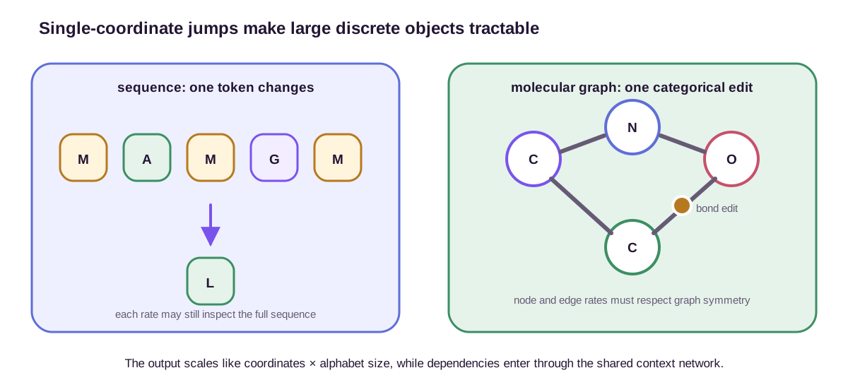
The restriction has a real cost. Suppose valid two-letter strings must have matching symbols, so only \(AA\) and \(BB\) are allowed. A single-site path from \(AA\) to \(BB\) must visit \(BA\) or \(AB\), both invalid. A coordinated rate \(q(BB\mid AA)\) can make the edit in one event, but it is absent from the factorized family. Molecular edits have the same shape: changing an atom’s formal charge and several incident bond orders may be valid as a coordinated transformation but invalid in every one-edit intermediate. Global context can correlate which single-site rate is large; it cannot make two sites jump simultaneously. One can add structured multi-coordinate events, constrain permitted transitions, or use corrector dynamics, but every richer event family increases the output space and complicates simulation.

Molecular graphs add symmetry to this tradeoff. Let \(\pi x\) denote the graph obtained by relabeling every node with permutation \(\pi\). A generator on labeled arrays represents a process on unlabeled graphs only if

\[q_t(\pi y\mid \pi x)=q_t(y\mid x).\]

For a node edit at index \(i\), the corresponding indexed statement is

\[q_t^{\pi(i)}(a\mid \pi x)=q_t^i(a\mid x),\]

with the analogous action on edge indices. This is a rate law, not merely an invariant graph-level prediction. To see what it buys, define \((T_\pi f)(x)=f(\pi^{-1}x)\). Substituting \(y=\pi z\) into the jump generator gives

\[\begin{aligned} (\mathcal{L}_tT_\pi f)(x) &=\sum_y q_t(y\mid x) \left[f(\pi^{-1}y)-f(\pi^{-1}x)\right]\\ &=\sum_z q_t(z\mid \pi^{-1}x) \left[f(z)-f(\pi^{-1}x)\right]\\ &=(T_\pi\mathcal{L}_tf)(x). \end{aligned}\]

Thus the generator commutes with relabeling. Equivalently, its finite-state rate matrix commutes with the permutation representation. An initial distribution invariant to relabeling remains invariant to relabeling under the master equation; this does not mean it is stationary in time. Variable-size generation still needs explicit birth, death, padding, or masking conventions, and the allowed event set itself must be closed under relabeling. Discrete flow matching has been adapted to graph generation with these constraints (Qin et al., 2025). The master equation does not guarantee chemical validity; validity enters through state representation, architecture, allowed jumps, training data, and possibly guidance.

Protein co-design reveals a second advantage. A protein combines discrete amino-acid identities with continuous translations and rotations. MultiFlow assigns a CTMC generator to sequence and geometric flows to structure, then learns them jointly (Campbell et al., 2024). This is difficult to express as a single vector field because the modalities do not share one tangent space. It is natural as a sum of generators on a product state space.

Generator matching unifies rather than flattens modalities

Suppose a state contains continuous coordinates, orientations, and categorical labels. Each component may have its own generator:

\[\mathcal{L}_t =\mathcal{L}_t^{\mathrm{flow}} +\mathcal{L}_t^{\mathrm{diffusion}} +\mathcal{L}_t^{\mathrm{jump}}.\]

Because the weak forward equation is linear in \(\mathcal{L}_t\), the sum is again a valid generator under suitable regularity conditions. The terms need not ignore one another: their coefficients may all condition on the full multimodal state. A sequence jump rate can depend on 3D geometry, while a geometric drift can depend on amino-acid identity.

For finite jump components, validity of the sum is almost visible: if \(Q^{(1)}\) and \(Q^{(2)}\) have nonnegative off-diagonal entries and zero column sums, then \(Q^{(1)}+Q^{(2)}\) has the same properties. In operator language, each component annihilates constants, \(\mathcal{L}^{(k)}1=0\), and satisfies the positive maximum principle; their sum does too. A diffusion term additionally needs a positive-semidefinite covariance, and drift or jump coefficients need the usual existence and non-explosion conditions. Cross-modal conditioning does not break this argument. It makes the coefficients state-dependent, but a geometry-conditioned jump kernel must still be nonnegative, and a sequence-conditioned diffusion tensor must still be positive semidefinite at every joint state.

The sum also has a pathwise interpretation. Competing clocks propose flow, diffusion, or jump increments over the same physical time axis. When a sequence rate depends on the current structure, a sequence event changes the drift used immediately afterward; superposition does not mean that the modalities evolve independently. It means that their infinitesimal contributions add before the forward equation is taken.

Conditional generator matching mirrors the discrete derivation. Construct a conditional generator \(\mathcal{L}_t^z\) that transports a simple source toward endpoint \(z\). The marginal generator acts as the posterior average

\[(\mathcal{L}_t f)(x) =\mathbb{E}\!\left[ (\mathcal{L}_t^Z f)(x) \mid X_t=x \right].\]

When the generator depends linearly on learnable coefficients—velocity, diffusion tensor, or jump kernel—conditional regression learns their marginal posterior average. The framework preserves what is different about each modality instead of embedding everything into a continuous surrogate and pretending every change is a vector displacement.

There is also non-uniqueness. A three-state circulation makes it explicit. On states \((A,B,C)\), let

\[Q_{\circlearrowright} =c\begin{pmatrix} -1&0&1\\ 1&-1&0\\ 0&1&-1 \end{pmatrix},\]

which sends \(A\to B\to C\to A\) at rate \(c\). The uniform marginal \(p=(1/3,1/3,1/3)^{\mathsf T}\) satisfies \(Q_{\circlearrowright}p=0\). The zero generator also satisfies \(0p=0\), as does the counterclockwise transpose \(Q_{\circlearrowright}^{\mathsf T}\). All three therefore preserve exactly the same one-time marginal for every \(t\).

Their paths are plainly different. Under the zero generator there are no events. Under the clockwise generator, the number of events in an interval of length \(T\) is Poisson with mean \(cT\), and an event from \(A\) always lands in \(B\); under the counterclockwise generator it lands in \(C\). Starting from the stationary ensemble hides this direction from every one-time histogram, but a signed edge-current measurement reveals flux \(c/3\) in opposite directions. Adding a circulation whose adjoint annihilates \(p_t\) can therefore change event count, temporal correlations, and simulation cost without moving the prescribed marginals.

This is also where the name “flow” needs discipline. A Generative Flow Network assigns nonnegative flow to edges of a directed construction graph so that incoming and outgoing construction flow balance and terminal probability is proportional to reward. Its graph is usually acyclic, its step index is not physical time, and its transition policies are normalized action probabilities. A CTMC generator may contain cycles, its off-diagonal entries have units of inverse time, and their sum determines an exponential waiting clock. The companion GFlowNet chapter develops DAG flow balance, detailed balance, and trajectory balance. Generator matching here concerns a different conservation law: \(\dot p_t=Q_tp_t\).

Simulation turns rates into an algorithmic tradeoff

Once rates are learned, there is no single obligatory sampler.

An event-driven sampler uses the total exit rate \(\lambda_t(x)\). For time-homogeneous rates, the waiting time is exponential with parameter \(\lambda(x)\), and the destination is drawn with probability

\[\Pr(Y=y\mid X=x,\text{jump}) =\frac{q(y\mid x)}{\lambda(x)}.\]

This Gillespie-style simulation represents individual events exactly. Time-dependent neural rates require inversion, thinning, or local approximations, and every accepted event may require another network evaluation. The method is accurate but inherently sequential.

For the analytic mask schedule, event-driven simulation is unusually simple: sample \(T=\kappa^{-1}(U)\) and then sample the destination. No numerical integration is needed. With learned, state-dependent rates, the integrated total hazard

\[H_x(t_0,t)=\int_{t_0}^{t}\lambda_s(x)\,ds\]

must reach an exponential threshold before the state changes. Quadrature, root finding, or thinning can require several network evaluations for one accepted event. “Exact event-driven” describes the stochastic construction when its hazard is evaluated exactly; it is not a promise of one neural evaluation per jump.

A fixed-step sampler chooses \(h\) and uses

\[\Pr(X_{t+h}=y\mid X_t=x) \approx \begin{cases} hq_t(y\mid x), & y\neq x,\\ 1-h\lambda_t(x), & y=x. \end{cases}\]

Validity requires \(h\lambda_t(x)\leq 1\). Smaller steps reduce first-order bias but increase the number of network evaluations. Updating several coordinates in parallel is fast on modern hardware, yet two nominally simultaneous changes omit the within-step dependence that a true CTMC would resolve sequentially. The resulting error is order \(h^2\) locally but can matter when rates are large or molecular constraints are tight.

The one-token example shows the boundary numerically. At \(t=0.9\), \(\lambda_t(M)=10\). A frozen Euler step of \(h=0.1\) has zero stay probability and forces a jump; \(h=0.2\) gives the invalid value \(1-h\lambda=-1\). The exact probability of jumping between \(t\) and \(t+h\) while still masked is

\[1-\exp\!\left(-\int_t^{t+h}\frac{ds}{1-s}\right) =\frac{h}{1-t}\]

for a linear schedule whose interval stays inside \([0,1]\). Here the Euler expression happens to equal the integrated result because \(1-\kappa_t\) is linear. That coincidence does not extend to a generic schedule or a learned rate.

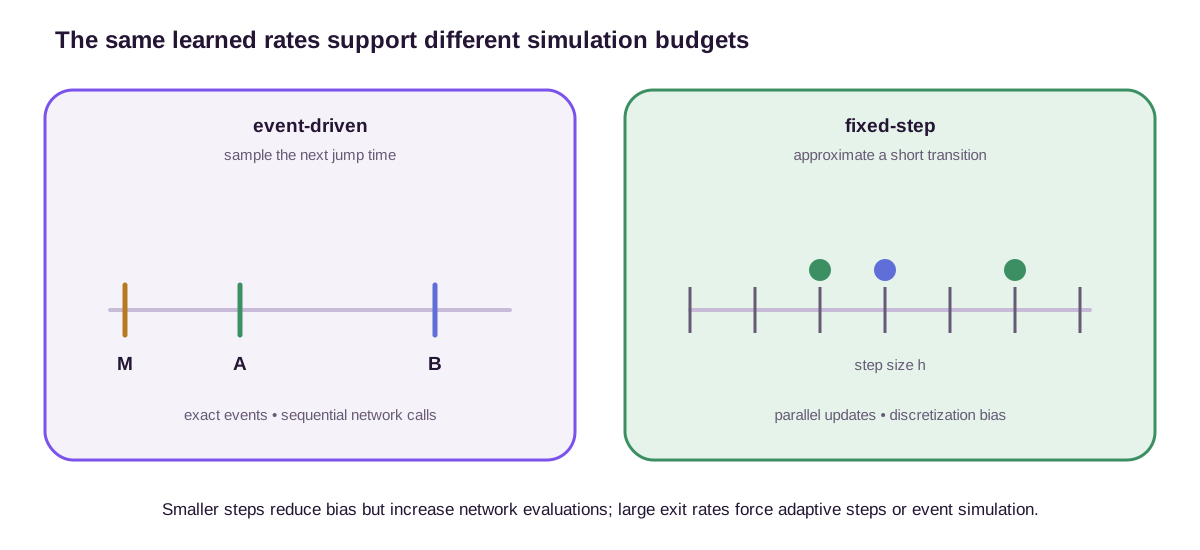
Adaptive steps, tau-leaping, predictor-corrector updates, and schedule redesign occupy the space between these extremes. The best choice depends on more than asymptotic correctness. Network evaluations, parallelism, endpoint stiffness, event sparsity, and the cost of invalid intermediate structures all matter.

One hundred masks: the NFE arithmetic

Return to the factorized model with \(d=100\) independently masked coordinates and \(\kappa_t=t\). Every coordinate jumps exactly once, so an exact event-driven trajectory contains exactly \(100\) accepted events. If the context network is recomputed after each edit, that is roughly \(100\) sequential network evaluations, plus any evaluations needed to integrate or bound a learned hazard. The expected number of still-masked coordinates is \(100(1-t)\), while each has rate \(1/(1-t)\). Their expected total exit rate is therefore

\[100(1-t)\frac{1}{1-t}=100.\]

Endpoint stiffness at the coordinate level does not make the expected aggregate event flux diverge.

A fixed grid with \(h=0.01\) uses \(100\) network evaluations whether a particular step edits zero coordinates or several. A coordinate still masked at \(t=0.99\) has jump probability one in the final interval. However, treating the whole sequence as a first-order CTMC step with at most one event would require \(h\lambda_t(x)\leq1\) for the total rate. Already at \(t=0\), \(h\lambda=0.01\times100=1\), and a realization with more surviving masks than its mean later can violate the bound. The global one-event approximation is therefore much more restrictive than the per-coordinate calculation.

Tau-leaping resolves this by sampling coordinate events in parallel from rates evaluated at the beginning of the interval. With \(h=0.02\), it uses \(50\) network evaluations and averages about two of the eventual \(100\) edits per step; with \(h=0.05\), it uses \(20\) evaluations and averages about five. For independent analytic masks, these Bernoulli updates can reproduce the correct interval law. For a learned context-dependent generator, all five edits in a coarse leap use stale pre-edit context. A valence change caused by the first edit cannot suppress an incompatible second edit inside the same leap. Reducing \(h\) restores sequential dependence at higher NFE; structured conflict resolution improves validity but changes the simulated kernel.

This arithmetic explains why sampler quality cannot be reported by NFE alone. Event-driven simulation spends evaluations where events occur and respects their order, but offers little batching. Tau-leaping amortizes one network call across many edits, but its error grows with both rate variation and interaction strength. Schedule design changes when events concentrate; event families change how many are needed; constraints change the cost of a stale update. The generator defines the ideal process, while the sampler defines which approximation to that process is actually deployed.

The central idea is therefore not that discrete data should imitate continuous trajectories. It is that both can be described infinitesimally. A vector field says how a point moves. A jump generator says how probability leaves one state and enters another. The master equation translates those local rates into a global probability path. Conditional paths make the otherwise intractable marginal generator learnable, and generator matching extends the construction without erasing the distinct geometry of each modality.

---

References

1. Campbell, A., Benton, J., De Bortoli, V., Rainforth, T., Deligiannidis, G., & Doucet, A. (2022). A continuous time framework for discrete denoising models. Advances in Neural Information Processing Systems, 35. ↩
2. Campbell, A., Yim, J., Barzilay, R., Rainforth, T., & Jaakkola, T. (2024). Generative flows on discrete state-spaces: Enabling multimodal flows with applications to protein co-design. Proceedings of the 41st International Conference on Machine Learning, 5453–5512. ↩
3. Gat, I., Remez, T., Shaul, N., Kreuk, F., Chen, R. T. Q., Synnaeve, G., Adi, Y., & Lipman, Y. (2024). Discrete flow matching. Advances in Neural Information Processing Systems, 37. ↩
4. Holderrieth, P., Havasi, M., Yim, J., Shaul, N., Gat, I., Jaakkola, T., Karrer, B., Chen, R. T. Q., & Lipman, Y. (2025). Generator matching: Generative modeling with arbitrary Markov processes. International Conference on Learning Representations. ↩
5. Qin, Y., Madeira, M., Thanou, D., & Frossard, P. (2025). DeFoG: Discrete flow matching for graph generation. Proceedings of the 42nd International Conference on Machine Learning, 50269–50326. ↩