Diffusion Models and Flow Matching

On this page

Adapted from my 2025 Machine Learning for Molecules and Geometric Deep Learning lectures. This article shows how score, noise, clean-data, and velocity prediction encode the same conditional path; the Fokker–Planck and probability-flow chapters provide the density and reverse-time background.

Two Ways to Learn Motion Through Probability Space

A generative model has to turn a simple distribution, usually a standard Gaussian, into a complicated data distribution. Diffusion models and flow-matching models appear to solve this problem differently. A diffusion model first destroys data with a stochastic process, learns the score of every intermediate noisy distribution, and then reverses the process. A flow-matching model specifies a probability path and learns the velocity field whose ordinary differential equation transports probability along it.

That distinction is real at sampling time, but it hides the more useful connection at training time. In both cases, the global object we need is an average over unknown data origins. The marginal score $\nabla_{\mathbf{x}}\log p_t(\mathbf{x})$ is unknown because the noisy marginal $p_t$ is unknown. The marginal flow velocity $\mathbf{u}_t(\mathbf{x})$ is unknown because it averages many conditional trajectories that can pass through the same point. Yet after conditioning on a clean data sample, both targets become elementary. Squared-error regression then performs the required marginalization automatically.

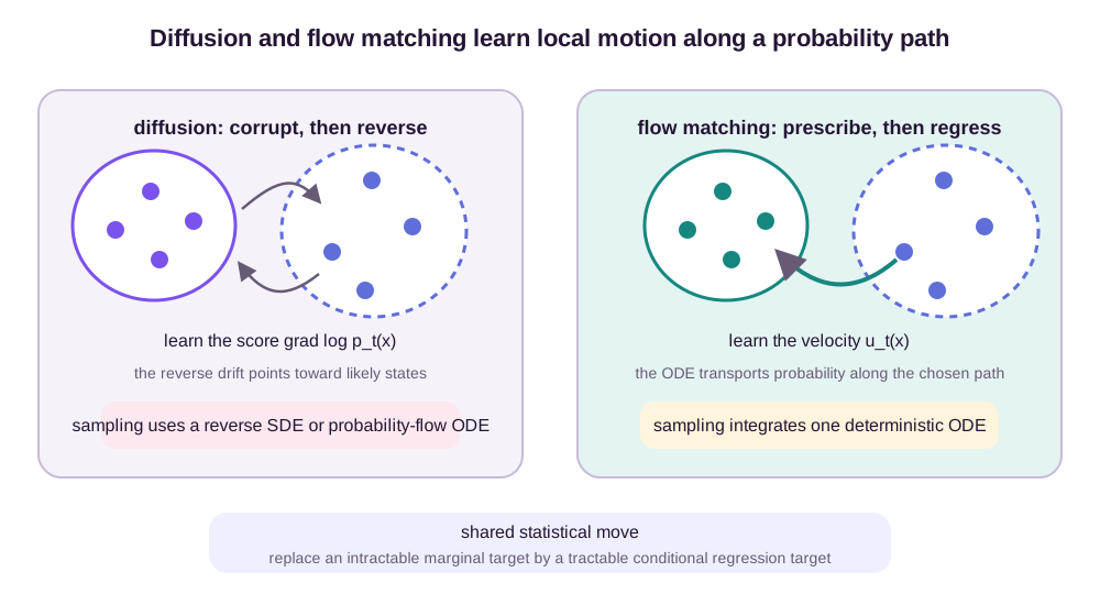
Diffusion and flow matching attach different local objects to an intermediate probability path: a score for reversing an SDE, or a velocity for integrating an ODE. Their training logic is shared: expose a tractable conditional target, then let regression recover its conditional mean at the observed state.

This is the thread of the post. We will first make corruption analytically tractable, derive denoising score matching, and use the learned score to reverse a diffusion. We will then prescribe conditional Gaussian paths, derive their velocities, and show why conditional flow matching learns the correct marginal ODE without simulating it during training. The final comparison separates the mathematical identities from the practical choices—schedule, prediction target, and numerical solver—that determine whether either model works well.

Throughout, time $t\in[0,1]$ is corruption time: $t=0$ is data and $t=1$ is the Gaussian base distribution. Diffusion naturally uses this convention. Many flow-matching papers instead put noise at $t=0$ and data at $t=1$; replacing $t$ by $1-t$ converts between the conventions and flips the velocity sign. Keeping one convention lets us compare the two methods without silently exchanging endpoints.

One deliberately non-Gaussian example will carry the argument. Let the data be the symmetric binary distribution

\[X_0\in\{-1,+1\}, \qquad \mathbb{P}(X_0=-1)=\mathbb{P}(X_0=+1)=\frac12,\]

and corrupt it by

\[X_t=\alpha_tX_0+\sigma_t\epsilon, \qquad \epsilon\sim\mathcal N(0,1).\]

Although the conditional kernels are Gaussian, the marginal is a two-component Gaussian mixture. It is simple enough to calculate exactly and complicated enough to expose the distinction between a conditional target and its marginal average. Every later formula will be checked on this same distribution.

Forward Corruption Makes a Hard Density Easy to Perturb

Let $\mathbf{x}_0\sim p_{\mathrm{data}}$. A continuous diffusion corrupts it through the Itô SDE

\[d\mathbf{X}_t = \mathbf{f}(\mathbf{X}_t,t)\,dt + g(t)\,d\mathbf{W}_t,\]

where $\mathbf{f}$ is a chosen drift, $g$ controls the noise rate, and $\mathbf{W}_t$ is Brownian motion. The coefficients are not learned. They are designed so that the terminal marginal $p_1$ is close to a distribution from which we can sample directly. Score-based SDE models make this construction explicit and derive both stochastic and deterministic reverse dynamics from the same intermediate marginals (Song et al., 2021).

The most convenient processes have a closed-form perturbation kernel. Their state at any time can be written

\[\mathbf{X}_t = \alpha_t\mathbf{X}_0 + \sigma_t\boldsymbol{\epsilon}, \qquad \boldsymbol{\epsilon}\sim\mathcal{N}(\mathbf{0},\mathbf{I}),\]

so that

\[p_{t|0}(\mathbf{x}\mid\mathbf{x}_0) =\mathcal{N}\!\left(\mathbf{x};\alpha_t\mathbf{x}_0,\sigma_t^2\mathbf{I}\right).\]

The boundary conditions $\alpha_0=1,\sigma_0=0$ preserve data, while $\alpha_1\approx0,\sigma_1\approx1$ erase it. Variance-preserving diffusions attenuate the signal while adding noise; variance-exploding diffusions primarily increase noise. Discrete denoising diffusion probabilistic models are time-discretized members of the same broad family (Ho et al., 2020).

The marginal at time $t$ is a mixture of these kernels:

\[p_t(\mathbf{x}) =\int p_{t|0}(\mathbf{x}\mid\mathbf{x}_0) p_{\mathrm{data}}(\mathbf{x}_0)\,d\mathbf{x}_0.\]

We can sample this mixture by drawing a data point and Gaussian noise. We generally cannot evaluate its density because the integral ranges over the entire data distribution. Diffusion training succeeds because it needs neither the density nor its normalization constant. It needs only the score, the spatial gradient $\nabla_{\mathbf{x}}\log p_t(\mathbf{x})$.

The binary mixture keeps the hidden origin visible

For the running example, the marginal density is

\[p_t(x) =\frac12\,\mathcal N(x;\alpha_t,\sigma_t^2) +\frac12\,\mathcal N(x;-\alpha_t,\sigma_t^2).\]

A positive observation is evidence for the $+1$ origin, but it does not identify that origin. Bayes’ rule makes the ambiguity quantitative. The posterior log odds are

\[\begin{aligned} \log\frac{p(X_0=+1\mid X_t=x)}{p(X_0=-1\mid X_t=x)} &=\frac{-(x-\alpha_t)^2+(x+\alpha_t)^2}{2\sigma_t^2}\\ &=\frac{2\alpha_tx}{\sigma_t^2}. \end{aligned}\]

If $m_t(x)=\mathbb E[X_0\mid X_t=x]$, then the sigmoid posterior and the identity $2\operatorname{sigmoid}(2z)-1=\tanh z$ give

\[m_t(x)=\tanh\!\left(\frac{\alpha_tx}{\sigma_t^2}\right).\]

This one hyperbolic tangent is the marginalization that the network must learn. Near the data endpoint, $\sigma_t$ is small and the posterior becomes almost binary except around $x=0$. Near the noise endpoint, $\alpha_t$ is small and the posterior mean collapses toward zero: the observation has forgotten which atom of the data distribution generated it. The marginal path therefore changes not only its variance but also its topology, from two separated modes toward one Gaussian-looking cloud.

Denoising Score Matching Is a Marginalization Identity

The conditional Gaussian score is known exactly:

\[\nabla_{\mathbf{x}}\log p_{t|0}(\mathbf{x}\mid\mathbf{x}_0) =-\frac{\mathbf{x}-\alpha_t\mathbf{x}_0}{\sigma_t^2}.\]

For a perturbed sample $\mathbf{x}_t=\alpha_t\mathbf{x}_0+\sigma_t\boldsymbol{\epsilon}$, this reduces to $-\boldsymbol{\epsilon}/\sigma_t$. The score points from the noisy observation back toward the mean of its particular corruption kernel. It is not yet the marginal score: two different clean samples can produce the same noisy location and suggest different directions.

Differentiate the mixture under the integral and divide by $p_t(\mathbf{x})$:

\[\begin{aligned} \nabla_{\mathbf{x}}\log p_t(\mathbf{x}) &=\frac{1}{p_t(\mathbf{x})} \int \nabla_{\mathbf{x}}p_{t|0}(\mathbf{x}\mid\mathbf{x}_0) p_{\mathrm{data}}(\mathbf{x}_0)\,d\mathbf{x}_0 \\ &=\int \nabla_{\mathbf{x}}\log p_{t|0}(\mathbf{x}\mid\mathbf{x}_0) p(\mathbf{x}_0\mid\mathbf{x})\,d\mathbf{x}_0 \\ &=\mathbb{E}\!\left[ \nabla_{\mathbf{x}}\log p_{t|0}(\mathbf{x}\mid\mathbf{X}_0) \mid \mathbf{X}_t=\mathbf{x}\right]. \end{aligned}\]

This denoising identity says that the marginal score is the posterior average of conditional scores. Crucially, training never has to calculate the posterior $p(\mathbf{x}_0\mid\mathbf{x}_t)$. Consider the loss

\[\mathcal{L}_{\mathrm{DSM}}(\theta) =\mathbb{E}_{t,\mathbf{x}_0,\boldsymbol{\epsilon}} \left[ \lambda(t)\left\| \mathbf{s}_\theta(\mathbf{x}_t,t) +\frac{\boldsymbol{\epsilon}}{\sigma_t} \right\|^2 \right].\]

At every fixed $(\mathbf{x}_t,t)$, the minimizer of squared error is the conditional mean of the target. It is therefore the marginal score. More precisely, the conditional-target loss equals a marginal-score regression loss plus the conditional variance of the target, which is independent of $\theta$. This is the score-matching–denoising connection developed by Vincent, 2011.

Why squared error performs the marginalization

The statement deserves a proof because several weaker claims are often called “equivalence.” Let $Y$ be any square-integrable conditional target, let $Z=(X_t,t)$ be what the network observes, and define $\mu(Z)=\mathbb E[Y\mid Z]$. For any predictor $h_\theta(Z)$,

\[\begin{aligned} \|h_\theta-Y\|^2 ={}&\|h_\theta-\mu\|^2+\|Y-\mu\|^2\\ &+2(h_\theta-\mu)^{\mathsf T}(\mu-Y). \end{aligned}\]

Condition on $Z$. The first factor in the cross term is fixed, while $\mathbb E[\mu-Y\mid Z]=0$. Therefore

The second term is the irreducible conditional variance and contains no $\theta$. If a nonnegative weight $\lambda(t)$ is used, the same proof works because that weight is measurable with respect to $Z$:

This is stronger than saying the losses have the same population minimizer. They differ by a parameter-independent constant, so their exact population gradients are identical under the usual differentiability and integrability conditions. It is also narrower: minibatch gradient variance differs because the conditional target is noisy, and a finite dataset or biased sampler need not realize the population expectation exactly.

For denoising score matching, take $Y=-(X_t-\alpha_tX_0)/\sigma_t^2$. Then $\mu(X_t,t)=\nabla_x\log p_t(X_t)$. For conditional flow matching later, take $Y=u_t(X_t\mid Z)$. The same theorem does both jobs; only the target changes.

The mixture score is a posterior-weighted compromise

The two possible conditional scores in the binary example are

\[s_t(x\mid x_0)=-\frac{x-\alpha_tx_0}{\sigma_t^2}, \qquad x_0\in\{-1,+1\}.\]

Averaging them with posterior mean $m_t(x)$ gives

\[s_t(x) =-\frac{x-\alpha_tm_t(x)}{\sigma_t^2} =-\frac{x-\alpha_t\tanh(\alpha_tx/\sigma_t^2)}{\sigma_t^2}.\]

At $x=0$, the two conditional scores point toward opposite mixture components and cancel. Away from zero, their posterior weights are unequal. The denoiser does not return to the particular source, which is unobserved; it averages the compatible returns given the noisy state.

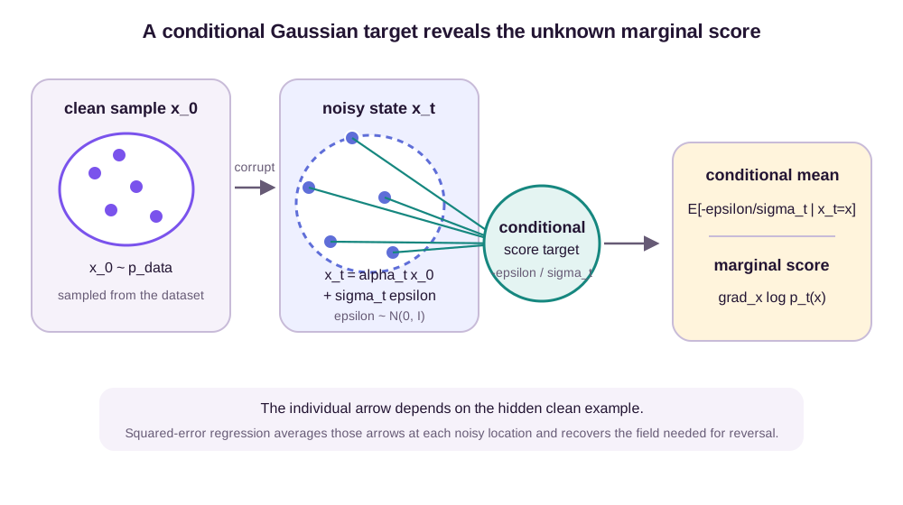
A Gaussian corruption gives the exact conditional score (-\epsilon/\sigma_t), but that arrow depends on the hidden clean sample. Averaging all compatible conditional arrows at a fixed noisy state yields the marginal score $\nabla_x\log p_t(x)$; squared-error regression performs this averaging without evaluating the posterior.

Implementations often predict $\boldsymbol{\epsilon}$, $\mathbf{x}_0$, or a linear combination called the velocity parameter rather than the score itself. These parameterizations contain equivalent information when $\alpha_t$ and $\sigma_t$ are known, but they scale errors differently across noise levels. The weight $\lambda(t)$ is therefore not cosmetic: together with the output parameterization, it decides which portions of the path dominate optimization.

The conversions make that claim precise. Away from endpoints where denominators vanish,

\[\widehat{\boldsymbol\epsilon}_\theta=-\sigma_t\mathbf{s}_\theta, \qquad \widehat{\mathbf{x}}_{0,\theta} =\frac{\mathbf{x}_t+\sigma_t^2\mathbf{s}_\theta}{\alpha_t} =\frac{\mathbf{x}_t-\sigma_t\widehat{\boldsymbol\epsilon}_\theta}{\alpha_t}.\]

Thus score, noise, and clean-data predictions are invertible representations of the same target information when $\alpha_t\sigma_t\neq0$. But unweighted losses are not identical. If $\mathbf{s}_\theta=-\widehat{\boldsymbol\epsilon}_\theta/\sigma_t$, then

\[\lambda_s(t)\|\mathbf{s}_\theta-\mathbf{s}\|^2 =\frac{\lambda_s(t)}{\sigma_t^2} \|\widehat{\boldsymbol\epsilon}_\theta-\boldsymbol\epsilon\|^2.\]

An unweighted noise loss equals a score loss weighted by $\sigma_t^2$, not an unweighted score loss. Likewise,

\[\lambda_s(t)\|\mathbf{s}_\theta-\mathbf{s}\|^2 =\lambda_s(t)\frac{\alpha_t^2}{\sigma_t^4} \|\widehat{\mathbf{x}}_{0,\theta}-\mathbf{x}_0\|^2.\]

These are identical weighted sample losses under the displayed conversions. Without transformed weights, one may still obtain the same pointwise conditional mean in an unconstrained function class, but the population norm, gradient magnitudes, finite-capacity compromise, and optimization trajectory change.

For a variance-preserving path with $\alpha_t^2+\sigma_t^2=1$, a useful rotated target is (Salimans and Ho, 2022)

\[\mathbf{v}=\alpha_t\boldsymbol\epsilon-\sigma_t\mathbf{x}_0.\]

The pair $(\mathbf{x}_t,\mathbf{v})$ is an orthogonal rotation of $(\mathbf{x}_0,\boldsymbol\epsilon)$, so

\[\mathbf{x}_0=\alpha_t\mathbf{x}_t-\sigma_t\mathbf{v}, \qquad \boldsymbol\epsilon=\sigma_t\mathbf{x}_t+\alpha_t\mathbf{v}.\]

At fixed $\mathbf{x}_t$, noise error is $\alpha_t$ times velocity-parameter error and data error is $-\sigma_t$ times it. An epsilon loss of weight $\lambda_\epsilon$ becomes a velocity loss of weight $\lambda_\epsilon\alpha_t^2$. The rotation stays bounded, but recovering the score still divides by $\sigma_t$. At $\sigma_t=0$ the data itself is observed and the score parameterization is singular; at $\alpha_t=0$ the conversion from $\mathbf{x}_t$ and a noise or score prediction to $\mathbf{x}_0$ divides by zero because the observation contains no source information. A direct $\mathbf{x}_0$ head does not itself divide by $\alpha_t$, but its endpoint target is nevertheless statistically unidentifiable from $\mathbf{x}_t$. Algebraic convertibility on the open interval does not erase endpoint conditioning.

The Score Turns Corruption Around

The forward SDE spreads probability. To generate, start at $\mathbf{X}_1\sim p_1$ and integrate back toward $t=0$. The reverse-time SDE is

\[d\mathbf{X}_t =\left[\mathbf{f}(\mathbf{X}_t,t) -g^2(t)\nabla_{\mathbf{x}}\log p_t(\mathbf{X}_t)\right]dt +g(t)\,d\overline{\mathbf{W}}_t, \qquad t:1\rightarrow0.\]

Here $dt$ is negative along numerical integration, and $\overline{\mathbf{W}}_t$ denotes reverse-time Brownian motion. The score correction compensates for the probability spreading of the forward noise. Replacing the unknown score by $\mathbf{s}_\theta$ produces the generative sampler.

The same marginal densities can also be generated by the probability-flow ODE

\[\frac{d\mathbf{X}_t}{dt} =\mathbf{f}(\mathbf{X}_t,t) -\frac{1}{2}g^2(t)\nabla_{\mathbf{x}}\log p_t(\mathbf{X}_t).\]

Why does the factor change from $1$ to $1/2$? The reverse SDE retains a diffusion term, which continues to spread density and needs the full score correction. The ODE has no random spreading, so half the correction produces the same Fokker–Planck evolution. This is an equality of one-time marginals, not of individual trajectories: stochastic and deterministic sample paths can look entirely different while visiting the same distributions at every time.

This already narrows the apparent gap to flow matching. Once a score is known, diffusion admits an ODE velocity. Flow matching asks whether we can train such a velocity directly, without first introducing an SDE or deriving its score.

Flow Matching Starts From a Conditional Path

An ODE

\[\frac{d\mathbf{X}_t}{dt}=\mathbf{u}_t(\mathbf{X}_t)\]

transports its marginal density according to the continuity equation

\[\partial_t p_t(\mathbf{x}) =-\nabla_{\mathbf{x}}\cdot \left[p_t(\mathbf{x})\mathbf{u}_t(\mathbf{x})\right].\]

If we knew a velocity field connecting data to noise, we could sample by integrating it backward. Directly designing the marginal path $p_t$ and solving for $\mathbf{u}_t$ is hard. Flow matching instead builds a family of easy conditional paths indexed by a condition $\mathbf{z}$—usually a data endpoint, or a paired data-and-noise endpoint—and then marginalizes them.

For a clean sample $\mathbf{x}_0$ and independent noise $\boldsymbol{\epsilon}$, use the same affine construction as above:

\[\mathbf{x}_t =\alpha_t\mathbf{x}_0+\sigma_t\boldsymbol{\epsilon}.\]

This equation now specifies an ODE trajectory rather than merely sampling the marginal of an SDE. Differentiate the trajectory:

\[\dot{\mathbf{x}}_t =\dot{\alpha}_t\mathbf{x}_0 +\dot{\sigma}_t\boldsymbol{\epsilon}.\]

The right-hand side is a tractable conditional velocity target. If we want it as a function of the current state and data endpoint, eliminate $\boldsymbol{\epsilon}=(\mathbf{x}_t-\alpha_t\mathbf{x}_0)/\sigma_t$:

\[\mathbf{u}_t(\mathbf{x}\mid\mathbf{x}_0) =\frac{\dot{\sigma}_t}{\sigma_t}\mathbf{x} +\left(\dot{\alpha}_t -\frac{\dot{\sigma}_t}{\sigma_t}\alpha_t\right)\mathbf{x}_0.\]

For the straight interpolation $\alpha_t=1-t$ and $\sigma_t=t$, every conditional trajectory moves at the constant velocity $\boldsymbol{\epsilon}-\mathbf{x}_0$ from data to noise. Generation integrates the learned field in the reverse direction. With the more common noise-to-data time convention, the same path is written $(1-t)\boldsymbol{\epsilon}+t\mathbf{x}_0$ and its velocity changes sign.

The binary path has an exact marginal velocity

For the affine Gaussian path, abbreviate

\[b_t=\frac{\dot\sigma_t}{\sigma_t}, \qquad c_t=\dot\alpha_t-\alpha_tb_t.\]

The conditional velocity is $u_t(x\mid x_0)=b_tx+c_tx_0$. Averaging over the binary posterior immediately gives

\[u_t(x)=b_tx+c_tm_t(x) =\frac{\dot\sigma_t}{\sigma_t}x +\left(\dot\alpha_t-\frac{\alpha_t\dot\sigma_t}{\sigma_t}\right) \tanh\!\left(\frac{\alpha_tx}{\sigma_t^2}\right).\]

The conditional trajectories are affine, but the marginal field is nonlinear because the posterior responsibility of each component changes with position. This is a useful warning about the word “straight”: straight conditional couplings do not imply a globally linear transport.

Take the variance-preserving trigonometric schedule

\[\alpha_t=\cos\frac{\pi t}{2}, \qquad \sigma_t=\sin\frac{\pi t}{2}.\]

At $t=1/2$, $\alpha_t=\sigma_t=1/\sqrt2$. For the observed state $x=0.5$,

\[m_t(0.5)=\tanh(1/\sqrt2)\approx0.6089,\]

so the posterior probabilities of origins $+1$ and $-1$ are about $0.8044$ and $0.1956$. Their conditional scores are

\[s_t(0.5\mid+1)=\sqrt2-1\approx0.4142, \qquad s_t(0.5\mid-1)=-(1+\sqrt2)\approx-2.4142.\]

The posterior average is $s_t(0.5)\approx-0.1389$. Meanwhile $b_t=\pi/2$ and $c_t=-\pi/\sqrt2$, so

\[u_t(0.5\mid+1)\approx-1.4360, \qquad u_t(0.5\mid-1)\approx3.0068,\]

and their posterior average is $u_t(0.5)\approx-0.5671$. One observed point therefore supports sharply different conditional motions. The marginal target is not either arrow; it is their responsibility-weighted current.

Conditional Velocities Produce the Correct Marginal Current

Suppose each conditional density $p_t(\mathbf{x}\mid\mathbf{z})$ satisfies a continuity equation with velocity $\mathbf{u}_t(\mathbf{x}\mid\mathbf{z})$. Its marginal is

\[p_t(\mathbf{x}) =\int p_t(\mathbf{x}\mid\mathbf{z})p(\mathbf{z})\,d\mathbf{z}.\]

Differentiate, insert the conditional continuity equation, and move the spatial divergence outside the integral:

\[\begin{aligned} \partial_t p_t(\mathbf{x}) &=-\nabla_{\mathbf{x}}\cdot \int \mathbf{u}_t(\mathbf{x}\mid\mathbf{z}) p_t(\mathbf{x}\mid\mathbf{z})p(\mathbf{z})\,d\mathbf{z} \\ &=-\nabla_{\mathbf{x}}\cdot \left[p_t(\mathbf{x}) \mathbb{E}[\mathbf{u}_t(\mathbf{x}\mid\mathbf{Z}) \mid\mathbf{X}_t=\mathbf{x}]\right]. \end{aligned}\]

Therefore a valid marginal velocity is

\[\mathbf{u}_t(\mathbf{x}) =\mathbb{E}\!\left[ \mathbf{u}_t(\mathbf{x}\mid\mathbf{Z}) \mid\mathbf{X}_t=\mathbf{x}\right].\]

This is the flow analogue of the denoising score identity. Conditional paths contribute probability currents, $p_t(\mathbf{x}\mid\mathbf{z})\mathbf{u}_t(\mathbf{x}\mid\mathbf{z})$. Their sum is the marginal current. Dividing by the marginal density turns that current into a posterior-weighted average velocity.

Many tractable conditional paths can overlap at the same state. Their probability-weighted currents add, so the marginal velocity is the posterior average $u_t(x)=\mathbb{E}[u_t(x\mid Z)\mid X_t=x]$; conditional flow matching learns this average without computing the posterior.

The ideal flow-matching objective would regress the neural field $\mathbf{u}_\theta$ onto this marginal velocity, but the posterior average is intractable. The conditional flow-matching objective is directly sampleable:

\[\mathcal{L}_{\mathrm{CFM}}(\theta) =\mathbb{E}_{t,\mathbf{z},\mathbf{x}\sim p_t(\cdot\mid\mathbf{z})} \left[ \left\|\mathbf{u}_\theta(\mathbf{x},t) -\mathbf{u}_t(\mathbf{x}\mid\mathbf{z})\right\|^2 \right].\]

Again, squared error returns the conditional mean at fixed $(\mathbf{x},t)$. The conditional loss differs from marginal velocity regression only by a $\theta$-independent variance term, so their gradients are identical. This gives simulation-free training: draw endpoints and a time, construct $\mathbf{x}_t$ in one algebraic step, compute its conditional velocity, and regress. No ODE trajectory has to be integrated during training. Flow matching formalized this construction for broad Gaussian paths and continuous normalizing flows (Lipman et al., 2023).

“Simulation-free” applies to training, not generation. Sampling still requires integrating the learned ODE from noise to data. It also does not mean the learned marginal trajectories are straight. Even when every conditional path is a straight line, their posterior average can bend because the set of plausible endpoints changes along the route.

The Common Core—and the Real Difference

The two regression identities can now be placed side by side:

\[\underbrace{\nabla\log p_t(\mathbf{x})}_{\text{marginal score}} =\mathbb{E}\!\left[ \underbrace{\nabla\log p_t(\mathbf{x}\mid\mathbf{X}_0)}_{\text{conditional score}} \mid\mathbf{X}_t=\mathbf{x}\right],\] \[\underbrace{\mathbf{u}_t(\mathbf{x})}_{\text{marginal velocity}} =\mathbb{E}\!\left[ \underbrace{\mathbf{u}_t(\mathbf{x}\mid\mathbf{Z})}_{\text{conditional velocity}} \mid\mathbf{X}_t=\mathbf{x}\right].\]

Both models choose a conditional probability path whose local target is tractable. Both train a neural network on samples from that path. Both rely on conditional expectation to recover a global field that is never evaluated directly. The distinction lies in what that field means.

The score describes the instantaneous geometry of a density: it points in the direction of greatest log-density increase. Combined with the known forward coefficients, it defines a reverse SDE and a probability-flow ODE. A flow-matching velocity directly describes probability transport: it specifies where states move so that the continuity equation follows the chosen path. A score alone is not a velocity, and a velocity need not be a score gradient. Diffusion connects them through a specific dynamical construction.

This also explains why “diffusion versus flow matching” is not a clean opposition. Flow matching can use diffusion probability paths. A diffusion score model can sample through a deterministic probability-flow ODE. The training target and sampling dynamics are modular choices, although changing one can alter conditioning and numerical error.

One affine path admits both derivations

The connection can be proved without repeating the Fokker–Planck derivation. Suppose $\alpha_t>0$ and define a linear forward SDE

\[dX_t=a_tX_t\,dt+g_t\,dW_t, \qquad a_t=\frac{\dot\alpha_t}{\alpha_t}.\]

Its conditional mean is $\alpha_tX_0$ when $\alpha_0=1$. To make its conditional variance equal $\sigma_t^2$, the variance equation must satisfy

\[\frac{d}{dt}\sigma_t^2=2a_t\sigma_t^2+g_t^2.\]

Hence the required diffusion rate is

\[g_t^2=2\sigma_t\dot\sigma_t-2a_t\sigma_t^2.\]

This construction is valid as a real scalar diffusion only where $g_t^2\geq0$. Not every visually plausible affine interpolation meets that condition. Ratios involving $\alpha_t$ or $\sigma_t$ also become singular at exact endpoints, so the formulas describe the open interval; implementations use limiting forms, non-divided parameterizations, or a small endpoint cutoff.

Now eliminate the posterior mean from the flow velocity. The mixture score identity implies

\[\alpha_tm_t(x)=x+\sigma_t^2s_t(x).\]

Substitute this into $u_t(x)=b_tx+c_tm_t(x)$:

\[\begin{aligned} u_t(x) &=\frac{\dot\alpha_t}{\alpha_t}x +\left(\frac{\dot\alpha_t}{\alpha_t}-\frac{\dot\sigma_t}{\sigma_t}\right) \sigma_t^2s_t(x)\\ &=a_tx-\frac12g_t^2s_t(x). \end{aligned}\]

The last line is exactly the forward-time probability-flow velocity of the linear SDE. The equality is pointwise in $(x,t)$ for the exact marginal score, so the induced ODEs are the same—not merely endpoint-equivalent. The SDE and ODE still have only matching one-time marginals, not matching transition kernels or path laws; that stronger distinction belongs to the companion probability-flow chapter.

For the trigonometric schedule, $a_t=-(\pi/2)\tan(\pi t/2)$ and

\[g_t^2=\pi\tan\frac{\pi t}{2}\geq0.\]

At $t=1/2$, $a_t=-\pi/2$ and $g_t^2=\pi$. Using the numeric mixture score above,

\[a_tx-\frac12g_t^2s_t(x) \approx-0.7854+0.2183=-0.5671,\]

which matches the posterior-averaged flow target. Diffusion and flow matching have arrived at the same field by different routes: one converts SDE probability current using a score, while the other averages conditional path velocities.

Equality of targets is not equality of training systems

There are now three distinct levels of equivalence. First, conditional and marginal squared-error objectives for the same network output differ by an exact parameter-independent variance term. Second, score, epsilon, data, and VP velocity targets contain invertibly related information inside the open interval. Third, their weighted losses become identical only after the schedule-dependent weights derived above are transformed as well.

Finite neural networks can break the practical correspondence. A shared architecture may represent $\epsilon(x,t)$ accurately but struggle with $s(x,t)=-\epsilon(x,t)/\sigma_t$ near small $\sigma_t$. Uniform time sampling combined with one target weights functions differently from uniform time sampling combined with another. Optimizer preconditioning, clipping, and finite minibatches further change the gradient noise. “Equivalent parameterizations” is therefore an algebraic statement unless the objective, weighting, function-class map, and endpoint treatment are also specified.

Schedules and Solvers Decide the Practical Model

The path schedule $(\alpha_t,\sigma_t)$ determines more than the pictures between the endpoints. It determines the conditional target magnitude, the signal-to-noise ratio seen by the network, how strongly different times are weighted, and whether the sampling dynamics become stiff near an endpoint. A schedule that changes almost nothing for most of the interval and then moves rapidly near $t=0$ forces a solver to resolve that narrow region. A straighter or more evenly parameterized path can often be traversed with fewer evaluations, but straight conditional paths do not guarantee a simple marginal field.

The neural parameterization changes the same conditioning. Score prediction divides the noise residual by $\sigma_t$ and can become large near the data endpoint. Noise prediction removes that division. Data prediction emphasizes reconstruction. Velocity parameterizations balance signal and noise differently. These are algebraically convertible only when the schedule is known; their optimization landscapes and finite-capacity errors are not identical.

A clock change preserves the path but rescales the problem

The geometric curve of distributions and the speed at which it is traversed are separate. Let $\tau=h(t)$ be a strictly increasing clock and write $t=h^{-1}(\tau)$. The reparameterized state $\widetilde X_\tau=X_{h^{-1}(\tau)}$ follows

\[\frac{d\widetilde X_\tau}{d\tau} =\frac{dt}{d\tau}\,u_t(\widetilde X_\tau).\]

Exact integration reaches the same distributions in the same order, so this is equality of the marginal curve after relabeling time. The regression target is multiplied by $dt/d\tau$, however, and uniform sampling in $\tau$ induces a nonuniform density over $t$. For example, $t=\tau^2$ gives velocity $2\tau u_{\tau^2}$. Uniform $\tau$ samples corruption time with density $q(t)=1/(2\sqrt t)$, allocating more examples near data. The same curve has become a different weighted training and integration problem.

The log signal-to-noise ratio makes the stiffness visible for the trigonometric schedule:

\[\rho(t)=\log\frac{\alpha_t^2}{\sigma_t^2} =2\log\cot\frac{\pi t}{2}, \qquad \dot\rho(t)=-\frac{2\pi}{\sin(\pi t)}.\]

At $t=0.5$, $$

\dot\rho

=2\pi\approx6.28$. At$t=0.99$, it is about$200$. If a fixed-step method is asked to keep the change$

\Delta\rho

\lesssim0.1$, the local step suggested by this crude criterion is about$0.0159$at the midpoint but only$0.0005$near$0.99$—roughly 32 times smaller. Uniform corruption-time steps spend resolution poorly. A clipped log-SNR clock expands the difficult endpoint region, though no finite clock includes the ideal endpoints where$\rho=\pm\infty$$.

This arithmetic also clarifies what “stiffness” means here. It is not simply that the data distribution is complicated. The schedule can make coefficients or their derivatives vary on sharply different time scales. A model may predict a statistically accurate target while a coarse solver misses the narrow interval in which that target changes most rapidly.

At sampling time, the solver introduces another approximation:

A reverse SDE sampler injects randomness at every step. Predictor–corrector or other stochastic schemes may improve exploration, but reproducibility and step allocation become additional choices.
A probability-flow or flow-matching ODE is deterministic for a fixed initial noise sample. Higher-order or adaptive solvers can reduce discretization error, but every function evaluation calls the neural network.
Fewer steps reduce cost but can skip regions where the vector field changes rapidly. More steps reduce integration error only until model error dominates.

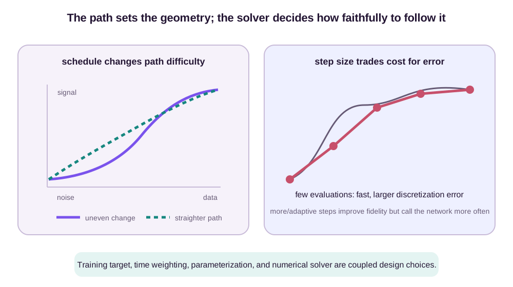
The schedule shapes where the probability path changes rapidly, while the numerical solver approximates motion along the learned field. Uneven or curved dynamics demand smaller or adaptive steps; increasing the number of network evaluations reduces discretization error but cannot repair an inaccurate learned target.

It is therefore misleading to attribute performance to the high-level framework alone. Noise schedule, time sampling, loss weighting, network preconditioning, target parameterization, and solver order interact. The diffusion design-space analysis of Karras et al., 2022 is valuable precisely because it separates these components rather than treating a sampler as an indivisible recipe.

An error contract from training target to generated sample

The exact identities provide a contract, not a promise that the implementation inherits them. It helps to audit five layers in order.

Target construction. The chosen conditional path, corruption kernel, analytic score, or conditional velocity must be correct. A sign error from exchanging data-to-noise and noise-to-data clocks changes the population target itself. A path that ends only approximately at the claimed base distribution also enters here as a design fact, not solver error.
Model regression. Finite capacity, finite data, and imperfect optimization make the network differ from the conditional mean. The MSE decomposition proves that conditional regression has the right population field, but its irreducible conditional variance still increases stochastic-gradient noise. It does not certify a trained finite network.
Time sampling and weighting. The model is fit in a weighted $L^2$ norm determined jointly by the time distribution, explicit loss weight, and output conversion. Reparameterizing time or switching from epsilon to score without compensating weights changes this norm. Regions receiving little mass can have large field error despite a small reported average loss.
Terminal prior. Exact reverse dynamics assume the starting sample is drawn from the actual terminal marginal $p_1$. If $\alpha_1$ is small rather than zero, the binary example ends in a Gaussian mixture, not exactly $\mathcal N(0,1)$. Replacing it by a standard Gaussian creates endpoint bias before the first solver step.
Numerical solver. The learned continuous field is finally discretized. ODE truncation error, SDE weak or strong error, tolerances, and endpoint cutoffs act on the model that was actually learned. More steps reduce this layer but do not repair the first four.

These errors are not generally additive scalars. A poorly sampled endpoint can produce a poorly learned field precisely where the solver is most sensitive; terminal mismatch can send samples into regions where the network was never trained. The contract is layered because downstream error depends on upstream state. A useful evaluation therefore reports target convention, time distribution, loss weighting, terminal approximation, and solver budget together rather than presenting one sample-quality number as a property of “diffusion” or “flow matching.”

The Lasting Unification

Diffusion and flow matching are best understood as two constructions of a learnable probability path. Diffusion chooses a forward stochastic process whose transition kernels are tractable. Denoising score matching turns their conditional scores into the marginal score, which supplies the missing reverse drift. Flow matching chooses tractable conditional paths directly. Conditional velocity regression turns their local motions into a marginal vector field, which supplies the ODE.

The binary mixture shows why this unification is more than analogy. At the same $(x,t)$, the hidden origins $-1$ and $+1$ produce different scores and different velocities. Bayes’ rule reduces both marginalizations to the same posterior statistic,

\[m_t(x)=\tanh\!\left(\frac{\alpha_tx}{\sigma_t^2}\right).\]

The marginal score uses it as $s_t(x)=-(x-\alpha_tm_t(x))/\sigma_t^2$; the marginal velocity uses it as $u_t(x)=b_tx+c_tm_t(x)$. When the affine path is realizable by the linear diffusion with $g_t^2\geq0$, substituting the first formula into the second gives the probability-flow velocity exactly. This chain has no appeal to visual similarity: posterior averaging, target regression, and probability current all identify the same pointwise field.

It also marks the boundary of the claim. The conditional DSM and marginal score losses are equal up to a constant only when they predict the same output under squared error. Score, epsilon, data, and VP velocity networks are algebraically convertible only away from singular endpoints. Their losses coincide only after weights are transformed. The SDE and its probability-flow ODE share one-time marginals, not trajectories. A flow with another divergence-free current could follow the same marginal curve by different paths. Naming the equality level prevents a useful unification from becoming a claim that every implementation is interchangeable.

The central trick is the same: design a conditional object that is easy to sample and differentiate, then use regression to marginalize over the hidden condition. Once that trick is visible, the field stops looking mysterious. The remaining questions are concrete engineering and modeling decisions: which path exposes a well-conditioned target, which parameterization distributes error sensibly over time, and which solver follows the learned dynamics accurately enough for the available compute.

References

Song, Y., Sohl-Dickstein, J., Kingma, D. P., Kumar, A., Ermon, S., & Poole, B. (2021). Score-Based Generative Modeling through Stochastic Differential Equations. International Conference on Learning Representations. ↩

Ho, J., Jain, A., & Abbeel, P. (2020). Denoising Diffusion Probabilistic Models. Advances in Neural Information Processing Systems, 33. ↩

Vincent, P. (2011). A Connection Between Score Matching and Denoising Autoencoders. Neural Computation, 23(7), 1661–1674. ↩

Lipman, Y., Chen, R. T. Q., Ben-Hamu, H., Nickel, M., & Le, M. (2023). Flow Matching for Generative Modeling. International Conference on Learning Representations. ↩

Karras, T., Aittala, M., Aila, T., & Laine, S. (2022). Elucidating the Design Space of Diffusion-Based Generative Models. Advances in Neural Information Processing Systems, 35. ↩

Salimans, T., & Ho, J. (2022). Progressive Distillation for Fast Sampling of Diffusion Models. International Conference on Learning Representations. ↩