On this page
Adapted from my 2025 Machine Learning for Molecules and Geometric Deep Learning lectures. This article develops the general principle behind equivariant models; Spherical Equivariant Layers carries that principle into three-dimensional architectures.
A geometric model should not spend parameters learning that a rotated molecule is still the same molecule. The coordinates have changed, but the object has not. If the target is energy, the prediction should stay fixed. If the target is force, the prediction should rotate with the atoms.
This observation sounds like data augmentation: rotate each training example and ask the network to fit all copies. But the stronger approach is to constrain the function itself. The model should give a consistent answer for every allowed transformation, including those absent from the training set. Geometry then becomes an architectural principle rather than a source of extra examples.
The same principle applies beyond molecules. Reordering the vertices of a graph changes its adjacency matrix but not the graph. Translating a point cloud changes every coordinate but not its internal shape. Shifting an image moves its pixels but preserves a local visual pattern. Each domain comes with transformations that change its description without changing the underlying object.
Geometry begins with a choice of sameness
Geometry specifies which properties survive a chosen class of transformations. Euclidean geometry, for example, studies distances and angles because rotations, translations, and reflections preserve them. For machine learning, the useful question is more operational: which transformations should leave the meaning of a data point unchanged? Bronstein et al. organize geometric deep learning around this domain-specific prior (Bronstein et al., 2021).
That question cannot be answered from coordinates alone. A molecule stored as an array contains both physical structure and arbitrary bookkeeping. Its row order is arbitrary, its origin is arbitrary, and its orientation is arbitrary. A model that treats these choices as signal sees many descriptions where a scientist sees one object.
The collection of descriptions connected by allowed transformations is called an orbit. The figure below shows a toy geometric graph under rigid motions and vertex relabeling. Each drawing belongs to the same orbit even though its coordinate array and row order differ.
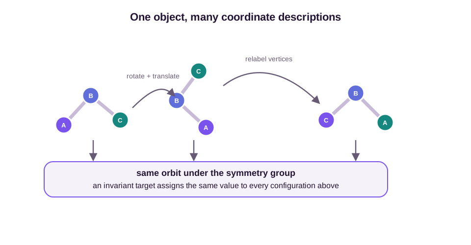
One V-shaped object, its orbit, and its stabilizer
A three-point object will carry the definitions. In two dimensions, place two identical type-A points and one type-B point at
\[\mathbf x_1=(-1,0),\qquad \mathbf x_2=(1,0),\qquad \mathbf x_3=(0,1).\]Call this ordered coordinate array \(X\), while remembering that the order of the two A points is bookkeeping. Let the allowed transformations be planar rigid motions together with permutations that exchange equal-type points. Translating the object by \((3,-2)\), rotating it by 40 degrees, or swapping rows 1 and 2 produces another description in the orbit \(G\cdot X=\{g\cdot X:g\in G\}\).
An orbit answers “which descriptions count as the same object?” A stabilizer answers the complementary question: “which transformations leave this particular description unchanged?” Formally,
\[G_X=\{g\in G:g\cdot X=X\}.\]The V has a nontrivial stabilizer. Reflecting across the vertical axis sends \(\mathbf x_1\) to \(\mathbf x_2\) and \(\mathbf x_2\) to \(\mathbf x_1\). If we simultaneously swap the two identical A rows, the stored typed configuration returns to itself. Thus the identity and this reflection-swap both belong to \(G_X\).
The stabilizer prevents a one-to-one correspondence between transformations and orbit points. If \(s\in G_X\), then \(g\cdot X=(gs)\cdot X\) even though \(g\) and \(gs\) are different transformations. More precisely, the orbit is isomorphic to the coset space \(G/G_X\). Symmetric objects have larger stabilizers and therefore fewer distinct poses than an asymmetric object under the same group.
The quotient space \(\mathcal X/G\) collapses each entire orbit to one point. An invariant target factors through this quotient: there exists a function \(\widetilde f\) such that
\[f(X)=\widetilde f([X]),\]where \([X]=G\cdot X\) denotes the orbit. This factorization is an exact identity once invariance is assumed. It says nothing about how to compute a good coordinate for \([X]\).
Why canonicalization fails at the stabilizer
One might try to represent the quotient by choosing one canonical description from each orbit. Center the V, align its covariance eigenvectors with the coordinate axes, and sort its A points lexicographically. Centering is safe because the centroid is unique. Principal-axis alignment is not.
For the centered V, the long principal axis is the horizontal line. An eigenvector specifies that line but not its sign: both \((1,0)\) and \((-1,0)\) are valid. The reflection-swap stabilizer exchanges these choices while leaving the physical object unchanged. A rule such as “make point 1 have positive horizontal coordinate” depends on which identical A point happened to receive row 1.
The degeneracy becomes sharper in a continuous family. Move the apex to \(\mathbf x_3=(0,h)\). At \(h=\sqrt3\), the three points form an equilateral triangle and the two covariance eigenvalues are equal. For \(h<\sqrt3\), the major principal axis is horizontal; for \(h>\sqrt3\), it is vertical. A PCA frame therefore jumps by 90 degrees as an arbitrarily small change in \(h\) crosses the degenerate configuration. A lexicographic sort can also swap row correspondence when a sign tie-break flips.
The obstruction here is narrow but consequential: at a nontrivial stabilizer, a unique frame-valued choice of group element cannot remain continuous through this PCA degeneracy. It is not a universal claim that quotient coordinates must be discontinuous. Distances provide continuous invariant coordinates for many point sets, and some restricted object families admit stable canonical representatives. Equivariance avoids committing the architecture to a fragile single-frame PCA-and-sorting rule: every pose remains valid, and predictions are related algebraically.
A symmetry is therefore never just a property of the input. It is a claim about the task. Rotating a molecule should preserve its energy, but it should rotate its dipole moment. Permuting atoms of the same element should preserve molecular properties, but exchanging carbon with oxygen is not an allowed permutation. A reflection may be appropriate for an isolated potential-energy model, while a chirality-sensitive classifier must distinguish mirror images. Choosing the wrong symmetry discards real information.
Groups turn transformations into algebra
To constrain a function for all transformations, we need to know how transformations compose. A group is a set of transformations with four properties: two transformations can be composed, composition is associative, an identity transformation does nothing, and every transformation has an inverse.
The definition is abstract because the same algebra describes different domains. The symmetric group \(S_N\) contains all permutations of \(N\) objects. The rotation group \(SO(3)\) contains all orientation-preserving rotations in three dimensions. The Euclidean group \(E(3)\) adds translations and reflections, while the special Euclidean group \(SE(3)\) contains rotations and translations but excludes reflections.
Rigid motions form a semidirect product
For rigid motions, we can represent a group element as a pair \((\mathbf{R}, \mathbf{t})\). Here, \(\mathbf{R}\) is a rotation matrix and \(\mathbf{t}\) is a translation vector. Acting on a point \(\mathbf{x} \in \mathbb{R}^3\) gives
\[(\mathbf{R}, \mathbf{t}) \cdot \mathbf{x} = \mathbf{R}\mathbf{x} + \mathbf{t}.\]The group law follows from applying two rigid motions in sequence:
\[\begin{aligned} (\mathbf R_2,\mathbf t_2)\cdot \bigl((\mathbf R_1,\mathbf t_1)\cdot\mathbf x\bigr) &=\mathbf R_2(\mathbf R_1\mathbf x+\mathbf t_1)+\mathbf t_2\\ &=(\mathbf R_2\mathbf R_1)\mathbf x +(\mathbf R_2\mathbf t_1+\mathbf t_2). \end{aligned}\]Since this must equal the action of the composed pair, we obtain
\[(\mathbf{R}_2, \mathbf{t}_2)(\mathbf{R}_1, \mathbf{t}_1) = (\mathbf{R}_2\mathbf{R}_1, \mathbf{R}_2\mathbf{t}_1 + \mathbf{t}_2).\]The second translation is not simply added to the first. The first translation must also be rotated by \(\mathbf{R}_2\). This coupling is why it is useful to treat rigid motions as group elements rather than as an informal list of augmentations.
The identity is \((\mathbf I,\mathbf 0)\). To derive the inverse, solve
\[(\mathbf R^{-1},\mathbf u)(\mathbf R,\mathbf t) =(\mathbf I,\mathbf 0).\]The composition law gives translation \(\mathbf R^{-1}\mathbf t+\mathbf u\), so \(\mathbf u=-\mathbf R^{-1}\mathbf t\). Therefore
\[(\mathbf R,\mathbf t)^{-1} =(\mathbf R^{-1},-\mathbf R^{-1}\mathbf t).\]Rotations act on translations before the vectors are added. Algebraically, \(SE(3)=SO(3)\ltimes\mathbb R^3\) is a semidirect product, not the direct product \(SO(3)\times\mathbb R^3\). The derivation is exact. Treating rotations and translations as independent augmentations is an implementation shortcut, not the group law.
SO(3), O(3), SE(3), and E(3) answer different questions
The orthogonal group is
\[O(3)=\{\mathbf Q:\mathbf Q^{\mathsf T}\mathbf Q=\mathbf I\}.\]Every orthogonal matrix has determinant \(+1\) or \(-1\). The subgroup \(SO(3)\) keeps only determinant \(+1\) and contains proper rotations. Matrices with determinant \(-1\) include reflections and improper rotations. Adding translations yields
\[SE(3)=SO(3)\ltimes\mathbb R^3, \qquad E(3)=O(3)\ltimes\mathbb R^3.\]The difference becomes observable for chirality. Take four labeled points in three dimensions and define their signed volume
\[\chi =(\mathbf x_2-\mathbf x_1)\cdot \left[(\mathbf x_3-\mathbf x_1)\times (\mathbf x_4-\mathbf x_1)\right].\]Translation cancels from every difference. Under an orthogonal transformation \(\mathbf Q\), the scalar triple product obeys
\[\chi'=\det(\mathbf Q)\chi.\]Proper rotations preserve the sign, while reflections reverse it. Two enantiomers therefore lie in different \(SE(3)\) orbits but in the same \(E(3)\) orbit. An \(E(3)\)-invariant model cannot distinguish them. That restriction is correct for a parity-even target such as an isolated nonrelativistic energy, but wrong for a handedness label or a parity-sensitive response.
A group action specifies how a group transforms a particular space. The rotation group acts on coordinates by matrix multiplication. The permutation group acts on a matrix of node features by reordering its rows. If \(\mathbf{P}\) is a permutation matrix, node features \(\mathbf{H}\) transform as
\[\mathbf{H} \mapsto \mathbf{P}\mathbf{H}.\]The same permutation acts on an adjacency matrix \(\mathbf{A}\) by reordering both endpoints of every edge:
\[\mathbf{A} \mapsto \mathbf{P}\mathbf{A}\mathbf{P}^{\mathsf{T}}.\]The input is one object, but its components transform in different ways. Coordinates, node features, edges, and targets therefore need separate actions.
A three-node graph makes the two actions concrete. Suppose the rows of \(\mathbf{H}\) store features for nodes \((1,2,3)\), and a permutation changes the stored order to \((3,1,2)\). Multiplication by \(\mathbf{P}\) performs exactly this row reordering. Each entry \(A_{ij}\) describes a pair of nodes, so the same relabeling must act on both indices; this gives \(\mathbf{P}\mathbf{A}\mathbf{P}^{\mathsf{T}}\). The transformed matrices may look different, but every edge still connects the same pair of physical nodes.
Now consider one message-passing update:
\[\mathbf{h}'_i = \phi\!\left( \mathbf{h}_i,\, \sum_{j \in \mathcal{N}(i)} \psi(\mathbf{h}_i,\mathbf{h}_j) \right).\]Here, \(\psi\) constructs a message from neighbor \(j\), the sum aggregates all incoming messages, and \(\phi\) updates node \(i\). The functions \(\phi\) and \(\psi\) are shared across nodes, while the sum ignores neighbor order. Relabeling the input therefore only relabels the outputs: \(\mathbf{H}' \mapsto \mathbf{P}\mathbf{H}'\). Permutation equivariance is not an emergent property of training; it follows from weight sharing and symmetric aggregation.
The layer-by-layer proof appears in Graph Neural Networks as Learnable Message Passing. Permutation equivariance is one instance of the same commuting constraint used below for rotations and rigid motions.
Representations describe how features transform
A group action on a vector space is called a representation when every transformation acts linearly. A representation \(\rho\) assigns a matrix \(\rho(g)\) to each group element \(g\) and preserves composition:
\[\rho(g_2g_1) = \rho(g_2)\rho(g_1).\]Representations are not an extra symmetry imposed on the data. They are the bookkeeping system that states how each quantity responds to a symmetry already chosen for the task.
Three homomorphisms verify the bookkeeping
The composition rule is a condition to check, not a naming convention. For permutations, choose the matrix convention
\[\mathbf P(\pi)\mathbf e_i=\mathbf e_{\pi(i)},\]where \(\mathbf e_i\) is basis vector \(i\). Applying \(\pi_1\) and then \(\pi_2\) gives
\[\mathbf P(\pi_2)\mathbf P(\pi_1)\mathbf e_i =\mathbf e_{\pi_2(\pi_1(i))} =\mathbf P(\pi_2\circ\pi_1)\mathbf e_i.\]Equality on every basis vector proves \(\mathbf P(\pi_2\circ\pi_1)=\mathbf P(\pi_2)\mathbf P(\pi_1)\). The permutation matrices therefore form a representation of \(S_N\).
For polar vectors under \(O(3)\), take \(\rho_{\mathrm{vec}}(\mathbf Q)=\mathbf Q\). Matrix multiplication immediately gives
\[\rho_{\mathrm{vec}}(\mathbf Q_2\mathbf Q_1) =\mathbf Q_2\mathbf Q_1 =\rho_{\mathrm{vec}}(\mathbf Q_2) \rho_{\mathrm{vec}}(\mathbf Q_1).\]For a rank-two tensor, define \(\rho_2(\mathbf Q)\mathbf T=\mathbf Q\mathbf T\mathbf Q^{\mathsf T}\). Two transformations give
\[\begin{aligned} \rho_2(\mathbf Q_2)\rho_2(\mathbf Q_1)\mathbf T &=\mathbf Q_2(\mathbf Q_1\mathbf T\mathbf Q_1^{\mathsf T})\mathbf Q_2^{\mathsf T}\\ &=(\mathbf Q_2\mathbf Q_1)\mathbf T (\mathbf Q_2\mathbf Q_1)^{\mathsf T}\\ &=\rho_2(\mathbf Q_2\mathbf Q_1)\mathbf T. \end{aligned}\]These are exact homomorphism checks. A learned layer may approximate an unknown physical function, but the transformation law of its declared feature types should not be approximate.
Three feature types cover much of what appears in geometric neural networks. A scalar does not change under rotation, so its representation is the number one. Energy, mass, and atom type are common scalar features. An ordinary vector transforms with the rotation matrix itself. Positions, velocities, forces, and electric fields are vector quantities. A rank-two Cartesian tensor, such as a stress tensor, transforms on both indices:
\[\mathbf{T} \mapsto \mathbf{R}\mathbf{T}\mathbf{R}^{\mathsf{T}}.\]The term steerable feature covers any feature vector whose components mix through a known representation matrix. Scalars, ordinary vectors, and higher-order tensor features are all steerable features. The name emphasizes that after transforming the input, we can steer the feature to its new value without recomputing it from scratch.
Parity separates polar and axial features
Under \(SO(3)\), every orthogonal transformation has determinant \(+1\), so two different \(O(3)\) feature types can look identical. A polar vector such as displacement, velocity, electric field, or force transforms as
\[\mathbf v\mapsto\mathbf Q\mathbf v.\]An axial vector such as angular momentum or magnetic field gains an additional parity factor:
\[\mathbf a\mapsto\det(\mathbf Q)\mathbf Q\mathbf a.\]The cross product explains the difference. If \(\mathbf a=\mathbf u\times\mathbf v\) for two polar vectors, then
\[(\mathbf Q\mathbf u)\times(\mathbf Q\mathbf v) =\det(\mathbf Q)\mathbf Q(\mathbf u\times\mathbf v).\]For a proper rotation, polar and axial vectors both transform by \(\mathbf Q\). Under inversion \(\mathbf Q=-\mathbf I\), a polar vector changes sign while an axial vector does not. Treating both as the same three-channel type silently imposes the wrong reflection law.
Scalars also carry parity. An ordinary scalar \(s\) remains fixed under reflection. A pseudoscalar \(p\) transforms as \(p\mapsto\det(\mathbf Q)p\); the signed volume \(\chi\) above is one example. Higher-order steerable features likewise need both angular type and parity when the group is \(O(3)\). The later posts on steerable features and tensor products and spherical equivariant layers develop how such types are coupled without duplicating that machinery here.
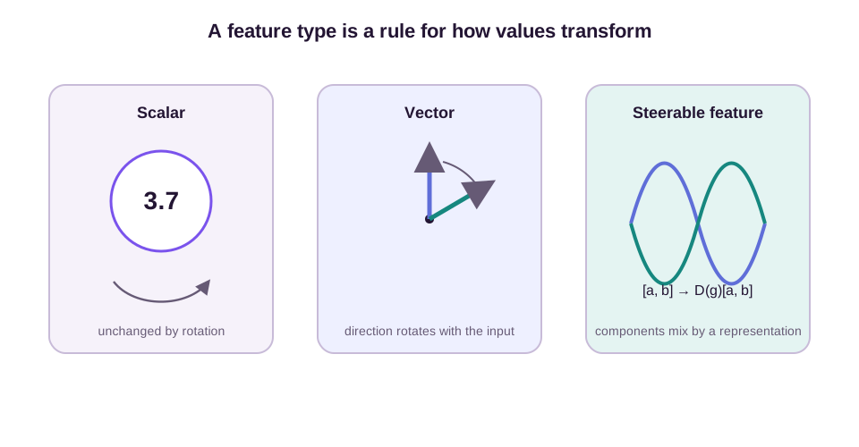
The transformation law matters more than the coordinate format. A three-dimensional array is not necessarily a geometric vector: three unrelated scalar channels should not rotate into one another. Conversely, a vector can be stored in a basis other than the Cartesian axes. Circular and spherical harmonics use coefficients whose components mix under rotations, yet they still carry precise geometric meaning. Their representation matrices make the transformation law explicit.
This distinction prevents a common modeling error. Applying an arbitrary multilayer perceptron to the three components of a force vector does not generally produce another vector. The nonlinear map can break the rotation law. Equivariant architectures restrict how different feature types mix so that every intermediate feature retains a defined transformation rule.
Invariance and equivariance constrain functions
Let \(f: X \rightarrow Y\) be a function from an input space \(X\) to an output space \(Y\). Suppose a group \(G\) acts on the input through \(\rho_X\) and on the output through \(\rho_Y\). The function is equivariant when
\[f\bigl(\rho_X(g)x\bigr) = \rho_Y(g)f(x) \qquad \text{for every } g \in G.\]The equation says that two computational paths agree. We can transform the input and then evaluate the function, or evaluate the function and then transform the output. The result must be the same.
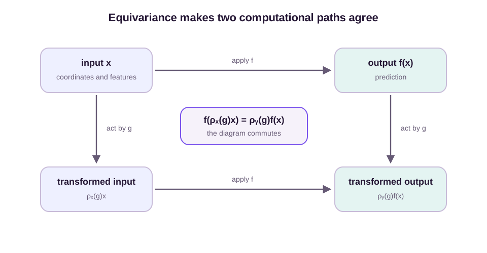
Invariance is a special case of equivariance. If the output should not change, then \(\rho_Y(g)\) is the identity and
\[f\bigl(\rho_X(g)x\bigr) = f(x).\]This compact equation separates the symmetry of a task into two decisions: how the input transforms and how the output transforms. The group alone is not enough. The same rotation group leads to invariance for energy and equivariance for force.
Equivariance is closed under composition
A network needs more than one valid layer. Suppose \(f:X\to Y\) is equivariant from representation \(\rho_X\) to \(\rho_Y\), and \(h:Y\to Z\) is equivariant from \(\rho_Y\) to \(\rho_Z\). Then
\[\begin{aligned} (h\circ f)(\rho_X(g)x) &=h\!\left(f(\rho_X(g)x)\right)\\ &=h\!\left(\rho_Y(g)f(x)\right)\\ &=\rho_Z(g)h(f(x))\\ &=\rho_Z(g)(h\circ f)(x). \end{aligned}\]The first and last lines use only function composition. The middle equalities use equivariance of \(f\) and \(h\). Therefore an arbitrary stack of equivariant primitives is equivariant. This closure theorem turns a layer-level contract into an architecture-level guarantee.
Addition is safe when both features have the same type:
\[\rho(g)(\mathbf u+\mathbf v) =\rho(g)\mathbf u+\rho(g)\mathbf v.\]Summing equivariant messages is safe for the same reason, while also removing neighbor order. Multiplying an equivariant feature by an invariant scalar is safe because \(s(\rho_X(g)x)=s(x)\):
\[s(\rho_X(g)x)\rho(g)\mathbf v =\rho(g)\bigl(s(x)\mathbf v\bigr).\]Readout must match the target. Norms and dot products turn polar vectors into invariants because orthogonal matrices preserve inner products. The trace of a tensor is invariant since
\[\operatorname{tr}(\mathbf Q\mathbf T\mathbf Q^{\mathsf T}) =\operatorname{tr}(\mathbf T).\]An equivariant vector readout can instead use invariant scalar weights:
\[\mathbf y=\sum_i\alpha_i\mathbf v_i, \qquad \alpha_i(\rho_X(g)x)=\alpha_i(x).\]Then \(\mathbf y\mapsto\mathbf Q\mathbf y\). Taking the norm of \(\mathbf y\) would be a safe final invariant readout, but it would destroy direction and cannot support a vector target.
Safe and unsafe nonlinearities
Pointwise nonlinearities are safe for scalar channels because scalars do not mix under rotation. They are generally unsafe for vector components. In two dimensions, take
\[\mathbf v=(1,-1), \qquad \mathbf R= \begin{bmatrix}0&-1\\1&0\end{bmatrix},\]where \(\mathbf R\) rotates by 90 degrees. Componentwise ReLU gives
\[\operatorname{ReLU}(\mathbf R\mathbf v) =\operatorname{ReLU}(1,1)=(1,1),\]whereas rotating the activated input gives
\[\mathbf R\operatorname{ReLU}(\mathbf v) =\mathbf R(1,0)=(0,1).\]The two paths disagree. No later equivariant layer can restore an exact guarantee already broken by this operation.
A radial nonlinearity is safe:
\[\Phi(\mathbf v) =\gamma(\lVert\mathbf v\rVert^2)\mathbf v,\]where \(\gamma\) is any learned scalar function. Since \(\lVert\mathbf Q\mathbf v\rVert^2=\lVert\mathbf v\rVert^2\),
\[\Phi(\mathbf Q\mathbf v) =\gamma(\lVert\mathbf v\rVert^2)\mathbf Q\mathbf v =\mathbf Q\Phi(\mathbf v).\]Gated nonlinearities use the same mechanism: an invariant scalar channel controls the magnitude of a vector or steerable channel. For a rank-two tensor, \(\mathbf T\mapsto\mathbf T^2\) is equivariant under the conjugation law because \((\mathbf Q\mathbf T\mathbf Q^{\mathsf T})^2=\mathbf Q\mathbf T^2\mathbf Q^{\mathsf T}\). Componentwise ReLU on the entries of \(\mathbf T\) is not. These are architectural identities; the particular gate or radial function is learned.
The distinction also appears in graphs. A graph-level prediction such as molecular solubility should be invariant to vertex ordering:
\[f(\mathbf{P}\mathbf{H}, \mathbf{P}\mathbf{A}\mathbf{P}^{\mathsf{T}}) = f(\mathbf{H}, \mathbf{A}).\]A node-level prediction such as an atom-wise charge should instead be permutation-equivariant:
\[f(\mathbf{P}\mathbf{H}, \mathbf{P}\mathbf{A}\mathbf{P}^{\mathsf{T}}) = \mathbf{P}f(\mathbf{H}, \mathbf{A}).\]The output values are physically unchanged, but their rows must follow the reordered atoms. Summation provides a simple invariant operation, while message passing with a shared update rule provides a simple equivariant operation. This is the algebraic reason graph neural networks share parameters across vertices and aggregate neighbors without using their order.
Euclidean symmetry combines several constraints. Let \(\mathbf{X} \in \mathbb{R}^{N \times 3}\) contain atomic coordinates as rows, and let \(\mathbf{F}(\mathbf{X})\) contain predicted forces. Under the row-vector convention, a rotation and translation act as
\[\mathbf{X} \mapsto \mathbf{X}\mathbf{R}^{\mathsf{T}} + \mathbf{1}\mathbf{t}^{\mathsf{T}}.\]An invariant energy model \(E\) and an equivariant force model \(\mathbf{F}\) should satisfy
\[E\!\left( \mathbf{X}\mathbf{R}^{\mathsf{T}} + \mathbf{1}\mathbf{t}^{\mathsf{T}} \right) = E(\mathbf{X}),\] \[\mathbf{F}\!\left( \mathbf{X}\mathbf{R}^{\mathsf{T}} + \mathbf{1}\mathbf{t}^{\mathsf{T}} \right) = \mathbf{F}(\mathbf{X})\mathbf{R}^{\mathsf{T}}.\]Translations disappear from the force transformation because forces have direction but no position.
Invariant energy produces equivariant forces and conservation laws
If forces come from the gradient of an invariant energy, rotational equivariance follows by the chain rule. Write the position and force of atom \(i\) as column vectors, and define
\[\mathbf F_i(X)=-\nabla_{\mathbf x_i}E(X).\]For \(Y=\{\mathbf y_i=\mathbf Q\mathbf x_i+\mathbf t\}\), energy invariance gives \(E(Y)=E(X)\). Perturb atom \(i\) by \(\delta\mathbf x_i\). The corresponding transformed perturbation is \(\delta\mathbf y_i=\mathbf Q\delta\mathbf x_i\). Equality of the two energy differentials requires
\[\nabla_{\mathbf y_i}E(Y)^{\mathsf T} \mathbf Q\delta\mathbf x_i =\nabla_{\mathbf x_i}E(X)^{\mathsf T} \delta\mathbf x_i\]for every perturbation \(\delta\mathbf x_i\). Therefore
\[\mathbf Q^{\mathsf T}\nabla_{\mathbf y_i}E(Y) =\nabla_{\mathbf x_i}E(X),\]and multiplying by \(\mathbf Q\) gives
\[\mathbf F_i(Y)=\mathbf Q\mathbf F_i(X).\]This is exact when the computed force is the exact derivative of an exactly invariant differentiable energy. A separately trained vector head may be equivariant but need not be conservative, because equivariance alone does not imply that the field is an energy gradient.
Continuous symmetries also produce zero-sum identities. Translation invariance means that for any vector \(\mathbf a\),
\[0=\left.\frac{d}{d\varepsilon} E(\{\mathbf x_i+\varepsilon\mathbf a\}) \right|_{\varepsilon=0} =-\mathbf a\cdot\sum_i\mathbf F_i.\]Since the equality holds for every \(\mathbf a\),
\[\sum_i\mathbf F_i=\mathbf 0.\]Infinitesimal rotation by vector \(\boldsymbol\omega\) moves each atom by \(\delta\mathbf x_i=\boldsymbol\omega\times\mathbf x_i\). Rotation invariance gives
\[0=-\sum_i\mathbf F_i\cdot (\boldsymbol\omega\times\mathbf x_i) =-\boldsymbol\omega\cdot \sum_i\mathbf x_i\times\mathbf F_i.\]Thus the net torque vanishes:
\[\sum_i\mathbf x_i\times\mathbf F_i=\mathbf 0.\]The first identity is conservation of total internal force; the second is conservation of internal torque. External fields or fixed supports break the corresponding symmetry and add external force or torque terms.
Consider a water molecule as a concrete case. Place the oxygen at the origin and the two hydrogens in the \(xy\)-plane. A rigid rotation changes all three coordinate rows, yet the O–H distances and H–O–H angle stay fixed. An energy model should return the same scalar before and after the rotation. Its force on each atom should preserve magnitude and rotate by the same matrix as the molecule. A model that predicts the correct energy but leaves its force vectors fixed in the laboratory frame is not physically consistent.
Relative displacements remove translations without discarding rotations:
\[\mathbf{r}_{ij} = \mathbf{x}_j - \mathbf{x}_i, \qquad \mathbf{r}_{ij} \mapsto \mathbf{R}\mathbf{r}_{ij}.\]Their lengths \(\lVert\mathbf{r}_{ij}\rVert\) are invariant, while the displacements themselves are equivariant vectors. A distance-only model can build an invariant energy from the lengths. A vector-aware model can also propagate directional information through \(\mathbf{r}_{ij}\). The second design is necessary when pairwise distances alone fail to distinguish configurations relevant to the target.
Architectural symmetry changes the hypothesis class
An unconstrained neural network searches over many functions that disagree on symmetry-related inputs. An equivariant architecture removes those functions before training. Its hypothesis class—the set of functions it can express—is smaller, but every remaining function respects the chosen transformation law.
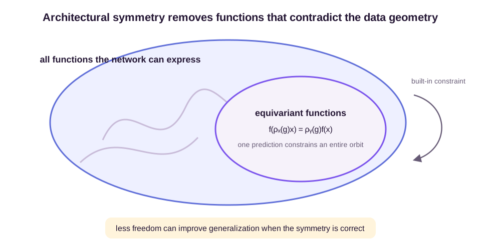
Convolutional networks provide the familiar case. A standard convolution applies the same filter at every image location, so translating the input translates the feature map. Group-equivariant convolutions extend this construction from translations to larger transformation groups (Cohen and Welling, 2016). Geometric graph networks follow the same design logic on permutations and continuous rotations, although their equivariant operations need not look like image convolutions.
There are three common ways to impose a symmetry, and they make different guarantees. The first is to build invariant inputs, such as pairwise distances. This route is simple, but any information removed by the invariant map is unavailable downstream. The second is to use equivariant intermediate features and equivariant layers, then convert to invariants only when the target requires them. This route preserves more information but requires representation-aware operations. The third is to average an arbitrary predictor over transformed inputs.
Group averaging projects a predictor onto equivariant functions
For a finite group, define
\[\overline f(x) =\frac{1}{\lvert G\rvert} \sum_{g\in G}\rho_Y(g^{-1}) f(\rho_X(g)x).\]The inverse output action transports each prediction back to the frame of the original input before averaging. To prove equivariance, transform the input by \(h\in G\):
\[\overline f(\rho_X(h)x) =\frac{1}{\lvert G\rvert} \sum_{g\in G}\rho_Y(g^{-1}) f(\rho_X(gh)x).\]Substitute \(k=gh\). As \(g\) ranges over the group, so does \(k\), and \(g^{-1}=hk^{-1}\). The representation law gives
\[\begin{aligned} \overline f(\rho_X(h)x) &=\frac{1}{\lvert G\rvert} \sum_{k\in G}\rho_Y(hk^{-1}) f(\rho_X(k)x)\\ &=\rho_Y(h)\overline f(x). \end{aligned}\]For an invariant output, \(\rho_Y(h)=1\) and the same construction becomes orbit averaging. The proof is an exact finite sum; it does not depend on learned parameters.
For a compact continuous group such as \(SO(3)\), the normalized Haar measure \(\mu\) replaces the finite average:
\[\bar{f}(x) = \int_G \rho_Y(g)^{-1} f\!\left(\rho_X(g)x\right)\,d\mu(g),\]Right-invariance of Haar measure, \(d\mu(gh)=d\mu(g)\), makes the same change-of-variables proof go through. Compactness matters because it permits a finite normalized measure. The translation group \(\mathbb R^3\) is noncompact, so it has no uniform probability distribution over all translations; one usually removes translations with relative coordinates or builds translation equivariance directly.
Exact integration over \(SO(3)\) is rarely available for an arbitrary neural predictor. Monte Carlo averaging over \(K\) sampled rotations is an approximation whose variance decreases with \(K\), but every forward pass still has sampling error and costs \(K\) evaluations. An equivariant architecture enforces the relation algebraically in one evaluation.
Four augmented poses do not imply continuous rotation invariance
A numerical example separates finite augmentation from an exact constraint. Let the target on the unit circle be
\[y(x_1,x_2)=x_1^2+x_2^2=1.\]Suppose training augmentation uses only rotations by 0, 90, 180, and 270 degrees of the point \((1,0)\). The predictor
\[f_\varepsilon(x_1,x_2) =x_1^2+x_2^2+\varepsilon x_1x_2\]fits all four augmented points exactly because one coordinate is zero at every sampled pose. At 45 degrees, \(x_1=x_2=1/\sqrt2\), so
\[f_\varepsilon(1/\sqrt2,1/\sqrt2) =1+\frac{\varepsilon}{2}.\]With \(\varepsilon=0.4\), augmented training error is zero while the unseen orientation has error 0.2. Optimization may learn \(\varepsilon\approx0\) from enough data, but the samples do not force it. A radial architecture of the form \(\phi(x_1^2+x_2^2)\) is exactly \(O(2)\)-invariant for every parameter choice and every angle.
Even exact averaging over the four-element rotation subgroup guarantees only 90-degree symmetry, not all of \(SO(2)\). The polynomial \(x_1^4-6x_1^2x_2^2+x_2^4\) is invariant under quarter turns but changes from 1 at 0 degrees to \(-1\) at 45 degrees. The group used by the architecture, not the word “augmentation,” determines the guarantee.
This restriction changes how information propagates from data. After seeing one molecular conformation, an exactly equivariant model already knows how its prediction must transform under every rotation. An unconstrained model must infer that relation from augmented samples and optimization. Data augmentation can encourage symmetry, but finite augmentation does not make the learned function exactly equivariant between sampled transformations.
Under symmetry assumptions on the data distribution and loss, group averaging cannot increase expected risk and can strictly reduce it (Elesedy and Zaidi, 2021). Those assumptions are part of the theorem. If the data distribution, target, or observation process breaks the group, restricting the predictor can increase risk.
A wrong reflection symmetry has an irreducible error
The signed-volume example makes wrong symmetry quantitative. Consider a balanced dataset containing reflected tetrahedral pairs with labels
\[y(X)=\operatorname{sign}\chi(X)\in\{-1,+1\}.\]An \(O(3)\)-invariant predictor must satisfy \(f(X)=f(\mathbf QX)\) for a reflection \(\mathbf Q\), while the labels satisfy \(y(\mathbf QX)=-y(X)\). For one reflected pair, write their shared prediction as \(c\). The mean squared error is
\[\frac{(c-1)^2+(c+1)^2}{2}=c^2+1\ge1.\]The lower bound holds for every parameter choice and depth because it follows from the imposed invariance. This is an architectural collision, not failed training. Replacing \(O(3)\) invariance with \(SO(3)\) invariance, or exposing a pseudoscalar channel, removes the assumption that identified the two enantiomers.
Other symmetry violations require adding the missing context rather than merely shrinking the group. A surface breaks translation symmetry normal to the interface. An external electric field selects a preferred direction. A labeled anchor atom breaks permutation symmetry. If the field is part of the input, jointly rotating molecule and field may remain a valid symmetry even though rotating the molecule alone is not. The right architecture preserves transformations of the complete task, not transformations of an isolated coordinate array.
There is also a computational tradeoff. Invariant models based only on pairwise distances are simple and efficient, but distances can discard orientation and chirality. Models with vector or higher-order steerable features retain more geometric information, at the cost of more structured operations. The appropriate feature types depend on the output and on which geometric distinctions the target actually uses.
Equivariance also changes failure modes. An unconstrained model can violate a symmetry arbitrarily far from its training orientations. An equivariant model cannot make that particular mistake, but it can still fit the wrong invariant dependence—for example, the wrong relationship between bond length and energy. Symmetry removes a family of inconsistent solutions; it does not supply the missing chemistry, data coverage, or optimization.
Symmetry changes learning because it changes what counts as a possible function. Group actions state how inputs and outputs transform. Representations state how features transform. Equivariance then requires the model to respect both statements at every point in its domain. Once those choices are explicit, geometry stops being vague intuition and becomes a testable contract for an architecture.
References
- Bronstein, M. M., Bruna, J., Cohen, T., and Veličković, P. (2021). Geometric Deep Learning: Grids, Groups, Graphs, Geodesics, and Gauges. arXiv:2104.13478. ↩
- Cohen, T. S., and Welling, M. (2016). Group Equivariant Convolutional Networks. Proceedings of ICML, 2990–2999. ↩
- Elesedy, B., and Zaidi, S. (2021). Provably Strict Generalisation Benefit for Equivariant Models. Proceedings of ICML, 2959–2969. ↩