Protein Representation Learning Across Sequence and Structure

Adapted from my 2025 Machine Learning for Molecules and Geometric Deep Learning lectures. Rather than ranking encoders by size, this article asks which biological neighborhood an embedding exposes and what evidence supports its claimed generalization. The AlphaFold chapter develops the complementary geometry and confidence machinery.

A protein admits several valid descriptions. Its amino-acid sequence records a polymer and an evolutionary history. A multiple sequence alignment exposes variation within a family. A residue graph makes spatial contacts explicit. Backbone frames retain local pose, while a molecular surface places the representation where many interactions occur. These descriptions are coupled, but they are not equivalent.

That distinction matters because a representation determines both what a model can learn easily and how it can fail. A sequence model may infer fold from evolutionary regularities without representing an active-site geometry explicitly. A structure encoder may recognize a binding pocket while ignoring that the observed conformation is only one member of an ensemble. A multimodal encoder may align sequence and structure—or merely learn family identity from both.

The practical question is therefore not whether an embedding “understands proteins.” It is which information survives the encoder, which shortcuts predict the benchmark label, and how far the resulting readout transfers beyond homologs of the training set.

I will carry one controlled protein through the argument. Protein P is a hypothetical 60-residue metal-binding mini-domain. Residues 8, 11, and 42 form a three-residue metal-binding motif after folding; residue 55 forms a distal surface contact. P has three recorded relatives that will later expose the difference between family retrieval and mechanism. The numbers are constructed so every representation and evaluation decision can be computed. They are not measurements of a named natural family.

A representation chooses a neighborhood

Let a protein sequence be

\[\mathbf a=(a_1,\ldots,a_L), \qquad a_i\in\mathcal A,\]

where \(\mathcal A\) contains the amino-acid alphabet and any special tokens. A sequence encoder maps the chain to residue embeddings

\[(\mathbf h_1,\ldots,\mathbf h_L) =f_{\theta}(a_1,\ldots,a_L).\]

Self-attention lets every position communicate with every other position, so the computational neighborhood is global along the chain. Yet the input itself contains no Cartesian coordinates. Geometry can only be inferred through statistical regularities learned from sequence data.

The same protein structure can be written as a residue graph

\[G=(V,E), \qquad V=\{1,\ldots,L\},\]

with edges defined by sequence adjacency, a distance cutoff, nearest neighbors, or a mixture of relations. Now spatial proximity is explicit, but it depends on the supplied conformation and on the graph construction. Two residues separated by 150 positions may become neighbors in a folded graph; two sequential neighbors remain connected even if a flexible loop moves them apart.

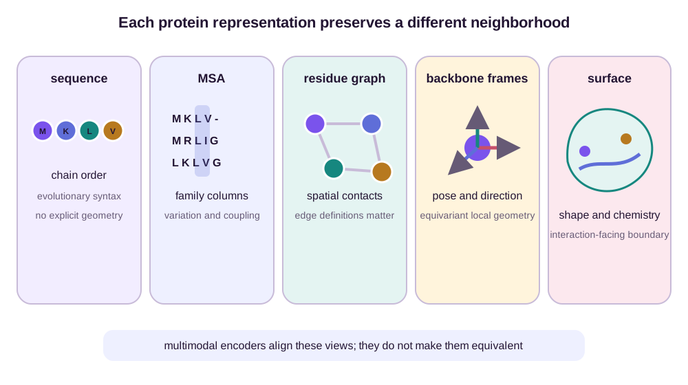
The choice is task-dependent. Chain order is indispensable for mutation likelihood and protein synthesis. Spatial contacts matter directly for catalytic pockets and interfaces. Surface geometry is often the most economical description of recognition by a partner. A universal representation that retains everything would be attractive, but it would also carry the cost and nuisance variation of every modality.

Protein P makes the neighborhoods concrete. In sequence, residue 8 is three steps from residue 11 but 34 steps from residue 42. A width-5 convolution expands its radius by two positions per layer, so information at 8 needs at least \(\lceil34/2\rceil=17\) layers to reach 42; global attention connects them in one layer, but must infer why that pair matters. In a folded residue graph with an \(8\,\text{\AA}\) cutoff, residues 8, 11, and 42 are mutual neighbors. One message layer can expose the complete metal-binding triad. The graph has made the mechanism computationally local by spending the supplied structure.

A backbone frame adds the orientation of the three coordinating side-chain directions, so it can distinguish a pocket whose pairwise distances are plausible but whose donors point away from the ion. A surface view hides buried residue 42 if the probe cannot enter the pocket, while emphasizing exposed residue 55. Mean pooling compresses all 60 residues into one vector and can dilute a three-residue signal by a factor of twenty. The same underlying protein therefore induces five different notions of “nearby,” each favorable to a different readout.

Sequence models learn evolutionary regularities from raw chains

Masked language modeling corrupts a subset \(M\) of residues and minimizes

\[\mathcal L_{\mathrm{MLM}} = -\sum_{i\in M} \log p_{\theta} \!\left(a_i\mid\widetilde{\mathbf a}\right),\]

where \(\widetilde{\mathbf a}\) is the corrupted sequence. To recover a buried residue, the model can use local motifs, long-range dependencies, family-level regularities, and biases in the sequence database. Scaling this objective to hundreds of millions of natural sequences produced representations in which structural and functional signals were readily accessible (Rives et al., 2021).

The evolutionary interpretation needs care. The training corpus is not a set of independent samples from a uniform protein universe. It contains phylogenetic correlations, unevenly sampled organisms and families, fragments, annotation artifacts, and many nearly redundant sequences. A language model compresses this observed distribution. Calling every regularity “biophysics” confuses the history of sampled life with the physical constraints acting on an isolated chain.

A common zero-shot mutation score is a log-odds difference at position \(i\):

\[s_i(a\rightarrow b) = \log p_{\theta}(a_i=b\mid\mathbf a_{\setminus i}) - \log p_{\theta}(a_i=a\mid\mathbf a_{\setminus i}).\]

This score asks whether the mutant looks more plausible under the learned sequence distribution. It is not a thermodynamic free-energy difference and not automatically a fitness effect. The two may correlate when evolutionary selection and the assay phenotype align; they can separate under novel environments, compensatory mutations, expression constraints, or functions absent from the training distribution.

At motif position 11 of P, suppose the masked model assigns histidine probability \(0.40\), glutamine probability \(0.10\), and the remaining mass to other residues. The zero-shot score for H11Q is

\[s_{11}(\mathrm H\rightarrow\mathrm Q) =\log 0.10-\log 0.40 =\log(0.25) \approx-1.386.\]

The model says glutamine is four times less probable than histidine in this sequence context. Multiplying by \(-RT\) would yield about \(0.82\,\mathrm{kcal\,mol^{-1}}\) at 298 K, but that number is not a mutation free energy. The language-model probabilities are normalized over sequence tokens, not conformational microstates in a thermodynamic ensemble. Database sampling, phylogeny, expression, and functional selection all contribute to them. Only an independently calibrated relation between log odds and a specified assay could turn the score into an empirical predictor for that assay.

The distinction changes decisions. H11Q might preserve the fold while removing a metal ligand; a family-trained model can penalize it because the residue is conserved. Conversely, a mutation that improves stability in a new solvent can receive negative log odds because evolution never sampled that environment. Sequence plausibility is evidence about the training distribution, not a universal energy oracle.

An MSA supplies a family coordinate system

A multiple sequence alignment is a matrix

\[\mathbf A\in(\mathcal A\cup\{\text{gap}\})^{M\times L},\]

whose rows are homologous sequences and whose columns are proposed corresponding positions. Row-wise attention models dependencies along each protein; column-wise attention compares variants at aligned sites across the family. MSA Transformer combines these two axes and learns contact-relevant patterns from masked prediction (Rao et al., 2021).

The alignment is powerful because evolution has already performed perturbation experiments. If substitutions at positions \(i\) and \(j\) co-vary across homologs, the residues may be structurally or functionally coupled. But raw covariance is also induced by shared ancestry and uneven sequence sampling. Alignment depth, search sensitivity, gap patterns, and family definition become part of the representation.

This makes an MSA a poor fit for some deployment settings. A new orphan sequence may have few detectable homologs. A rapidly evolving viral protein may sit outside the curated family. An engineered protein may deliberately combine motifs without a natural alignment history. Single-sequence language models trade explicit family statistics for an amortized prior learned across many families; they do not make evolutionary information disappear.

For P, compare a deep alignment of \(M=2{,}000\) raw rows with an orphan search returning only four sequences. If redundancy weighting gives each cluster total weight one, the deep alignment may have an effective sequence count \(M_{\mathrm{eff}}=320\). A residue-pair frequency estimated near \(0.10\) then has an independent-binomial standard error of roughly

\[\sqrt{\frac{0.10(0.90)}{320}}=0.0168.\]

With four effectively independent rows, the same approximation gives \(0.150\), nearly nine times larger. Phylogeny and gaps violate the binomial assumption, so these values are optimistic diagnostics rather than calibrated uncertainty. They still expose the regime change: column statistics that are stable in a deep family become individual anecdotes for an orphan.

The AlphaFold chapter explains how alignments and pair representations support structure prediction. For representation learning, the operational question is availability. If deployment supplies a deep MSA for P but none for a novel family Q, an MSA encoder and a single-sequence encoder did not receive comparable evidence. Results should be stratified by \(M_{\mathrm{eff}}\) or another declared depth measure rather than averaged across those cases.

Structure encoders must respect geometry and polymer order

A point cloud of residue coordinates is not yet a protein representation. It discards which atoms form each residue, how residues connect along the backbone, and which orientation a side chain presents. Structure encoders usually restore this relational information while enforcing the desired rigid-motion behavior.

For an invariant protein-level prediction \(y\), rotating and translating the coordinates should not change the output:

\[f(Q\mathbf X+\mathbf 1\mathbf t^{\top})=f(\mathbf X), \qquad Q\in SO(3).\]

Internal vector features should instead transform equivariantly. A geometric vector perceptron, for example, propagates scalar and vector channels together so direction can be retained without tying the result to an arbitrary laboratory frame (Jing et al., 2021).

Residue graphs offer an efficient compromise. A message-passing layer with relation-specific neighborhoods can be written as

\[\mathbf h_i^{(\ell+1)} = \mathbf h_i^{(\ell)} + \sum_{r\in\mathcal R} \sum_{j\in\mathcal N_r(i)} \phi_r^{(\ell)} \!\left(\mathbf h_i^{(\ell)},\mathbf h_j^{(\ell)},\mathbf e_{ij}\right).\]

Here \(r\) may denote sequential, radius, or nearest-neighbor edges. GearNet makes these relations explicit and also propagates between edges to encode angles; its geometric pretraining results show how a modest number of structures can yield transferable representations (Zhang et al., 2023). The point is not that one graph definition is canonical. It is that the edge set declares what counts as local before learning begins.

Backbone frames retain pose, not merely distance

Distances are invariant and useful, but distances alone hide orientation at an individual residue. A local backbone frame can be constructed from the nitrogen, alpha-carbon, and carbonyl-carbon atoms. Represent residue \(i\) by

\[T_i=(R_i,\mathbf t_i)\in SE(3),\]

where \(R_i\) is an orthonormal frame and \(\mathbf t_i\) is its origin. The relative pose of residue \(j\) in frame \(i\) is

\[T_i^{-1}T_j = \left(R_i^{\top}R_j, R_i^{\top}(\mathbf t_j-\mathbf t_i)\right).\]

This quantity is unchanged by a common global rigid transformation. It exposes whether two peptide planes face one another, not just how far apart their origins are. Such directional information matters for hydrogen-bond geometry, side-chain packing, and inverse folding.

Frames also introduce assumptions. Missing backbone atoms make a frame undefined. Experimental alternate conformations and predicted structures carry uncertainty. Chirality and reflection behavior must be handled deliberately. A model can be perfectly equivariant to rotations while being confidently wrong about an uncertain loop.

Relative pose and a chirality witness

Let residue 8 of P define \(R_8=I\) and origin \(\mathbf t_8=(0,0,0)\). Let residue 42 have origin \(\mathbf t_{42}=(2,1,0)\) and a frame rotated by \(90^\circ\) around \(z\),

\[R_{42}= \begin{pmatrix} 0&-1&0\\ 1&0&0\\ 0&0&1 \end{pmatrix}.\]

The pose of residue 42 as seen from residue 8 is simply \((R_{42},(2,1,0))\). Now rotate and translate the whole protein by \((Q,\mathbf b)\). The new frames are \(QR_i\) and the new origins are \(Q\mathbf t_i+\mathbf b\). Their relative translation is

\[(QR_8)^{\top} \left[(Q\mathbf t_{42}+\mathbf b)-(Q\mathbf t_8+\mathbf b)\right] =R_8^{\top}(\mathbf t_{42}-\mathbf t_8),\]

because \(Q^{\top}Q=I\). The translation cancels, and the relative rotation similarly becomes \(R_8^{\top}R_{42}\). Relative frames preserve pose without preserving a laboratory coordinate system.

Distances still cannot determine handedness. Take three unit directions from a local center, \(\mathbf u=(1,0,0)\), \(\mathbf v=(0,1,0)\), and \(\mathbf w=(0,0,1)\). Their signed triple product is

\[\chi=\mathbf u\cdot(\mathbf v\times\mathbf w)=1.\]

Reflect across the \(yz\) plane. Every pairwise distance remains unchanged, but \(\mathbf u'=(-1,0,0)\) gives \(\chi'=-1\). An architecture invariant to the full orthogonal group \(O(3)\) identifies these mirror configurations unless parity-sensitive features are supplied. Proteins use one amino-acid handedness, so reflection invariance can erase a chemically meaningful distinction even when rotation invariance is required.

Surfaces move the representation to the interaction boundary

Many molecular interactions occur through a solvent-excluded surface rather than at residue centers. A surface representation samples points

\[\mathcal S = \{(\mathbf p_k,\mathbf n_k,\mathbf c_k)\}_{k=1}^{K},\]

where \(\mathbf p_k\) is a surface position, \(\mathbf n_k\) its normal, and \(\mathbf c_k\) local chemical features such as hydrophobicity or electrostatic potential. Local patches can express curvature, charge complementarity, and exposed chemistry directly. MaSIF demonstrated that geometric surface fingerprints can support pocket and protein-interaction tasks (Gainza et al., 2020).

This view is especially natural for binding-site comparison across proteins with different folds. It is less natural for questions about chain synthesis, buried allostery, or conformational transitions. Surface generation also depends on probe radius, protonation, side-chain placement, and the chosen structure. The surface is an interaction-facing summary, not a lossless substitute for atoms.

Resolution changes both cost and the smallest visible feature. Suppose P has solvent-accessible area \(3{,}000\,\text{\AA}^2\). Sampling one point per \(4\,\text{\AA}^2\) yields about 750 points; one point per \(1\,\text{\AA}^2\) yields about 3,000. A local all-pairs patch calculation with 32 neighbors grows from roughly 24,000 to 96,000 directed interactions. The denser mesh can resolve a narrow groove that a four-square-angstrom sample skips, but it does not create certainty about side chains that were unresolved in the input structure.

Probe radius declares which cavities count as accessible. A water-like probe of radius \(1.4\,\text{\AA}\) cannot enter a hypothetical \(2.4\,\text{\AA}\)-wide neck because its diameter is \(2.8\,\text{\AA}\). A \(1.0\,\text{\AA}\) probe can. In P, residue 42 may therefore be absent from the first surface and exposed in the second, even though the atomic coordinates are identical. If the task concerns water exclusion, the larger probe is meaningful. If it concerns a smaller ion, it may delete the relevant pocket. Surface resolution and probe radius are physical modeling choices, not merely graphics settings.

Pretraining decides what becomes easy to read out

Representations are often judged by a downstream predictor, but the pretraining loss has already decided which distinctions the encoder is rewarded for preserving.

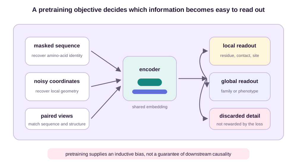
Structure pretraining can mask residue identities, predict distances or orientations, denoise coordinates, or contrast two augmented views. For a positive pair \((x_i,x_i^+)\) and negatives \(x_j^-\), a typical contrastive objective is

\[\mathcal L_i = -\log \frac{\exp(\operatorname{sim}(z_i,z_i^+)/\tau)} {\exp(\operatorname{sim}(z_i,z_i^+)/\tau) +\sum_j\exp(\operatorname{sim}(z_i,z_j^-)/\tau)}.\]

The augmentations define the intended invariance. Cropping teaches that local views of one structure should agree; it may erase domain arrangement. Coordinate noise rewards local geometric recovery; it may emphasize crystallographic regularity rather than function. Treating homologs as negatives can push biologically related proteins apart, while treating them as positives can collapse functionally meaningful variation within a family.

Multimodal learning adds another decision. Separate encoders may align a sequence embedding \(z_i^{\mathrm{seq}}\) with a structure embedding \(z_i^{\mathrm{str}}\), or a joint vocabulary may pair each residue with a discrete structure token. SaProt takes the latter route, training a language model over combined sequence and structure tokens (Su et al., 2024). This gives the sequence stack direct access to local structural states, but the tokens inherit the resolution and errors of the structure encoder that produced them.

Alignment does not imply equivalence. Sequence contains evolutionary and synthesis information absent from a single structure. Structure contains conformation-specific geometry absent from raw sequence. A useful joint representation may preserve their shared signal while retaining modality-specific channels instead of forcing every detail into one latent vector.

A finite contrastive batch declares invariance

Consider one anchor view of P, a cropped positive view, an unrelated negative U, and a homolog P1 placed in the negative set. Let cosine similarities to the anchor be \(0.8\) for the positive, \(0.2\) for U, and \(0.8\) for P1. With temperature \(\tau=0.2\), the three logits are \((4,1,4)\). The positive probability inside InfoNCE is

\[\frac{e^4}{e^4+e^1+e^4}=0.488, \qquad \mathcal L=-\log(0.488)=0.718.\]

If P1 were not treated as a negative, the probability would be \(e^4/(e^4+e^1)=0.953\) and the loss only \(0.049\). The large extra gradient does not arise because the encoder failed to match the two views of P. It arises because the batch construction demands that P separate from a close homolog. That demand may help instance retrieval and hurt family-level transfer.

The positive crop makes an equally consequential declaration. If the crop preserves only residues 1–30, it removes motif residue 42 yet the objective pulls its embedding toward the full protein. The encoder is rewarded for invariance to losing part of the metal-binding mechanism. A local-structure task may benefit from cropping; a function task may not. “Augmentation strength” is therefore shorthand for a biological equivalence relation imposed during training. A defensible objective states which transformations should preserve the target and tests a counterexample where they should not.

Protein-level pooling can erase the mechanism

Residue embeddings must often be converted into a protein embedding:

\[\mathbf z = \operatorname{Pool} \{\mathbf h_1,\ldots,\mathbf h_L\}.\]

Mean pooling is size-stable and simple, but a catalytic triad can vanish among hundreds of irrelevant residues. Sum pooling retains extensive counts but entangles them with length. A learned attention pool can focus on a motif, yet may instead select a taxonomic or localization signal correlated with the label.

The needed granularity follows the task. Residue-wise embeddings suit active-site and interface prediction. Pair embeddings suit contacts and mutation interactions. Domain embeddings suit modular proteins. A single global vector is convenient for retrieval, but convenience should not be mistaken for a mechanistic bottleneck.

Protein P gives a minimal pooling calculation. Project each residue embedding onto a motif direction and assign value 1 to residues 8, 11, and 42 and value 0 to the other 57 residues. Mean pooling returns

\[z_{\mathrm{mean}}=\frac{3}{60}=0.05,\]

whereas sum pooling returns \(z_{\mathrm{sum}}=3\). Append a 60-residue inert domain whose projections are all zero. The motif is unchanged, but the mean falls to \(3/120=0.025\). The sum stays 3, although on realistic nonzero backgrounds it also grows with length and repeated motifs.

Suppose an attention pool assigns weight \(0.20\) to each motif residue and spreads the remaining \(0.40\) over all background residues. Its motif coordinate is \(0.60\). Attention has avoided dilution only because a learned scorer already located the motif. If taxonomic family predicts the label more easily, the same capacity can focus on family-specific residues instead. Mean pooling builds in democratic averaging, sum pooling builds in extensivity, and attention pooling learns a selection rule. The downstream claim should match that rule rather than treating “protein embedding” as a neutral operation.

Structure leakage can arrive through several doors

“Structure-aware” evaluation is ambiguous when structure is predicted from sequence. Suppose the downstream test protein was absent from supervised training, but a close homolog appeared in the folding model’s training set, in the representation pretraining corpus, or in a template database. The supplied predicted structure can transmit that prior into the downstream model.

Leakage is not limited to identical PDB entries. The following can cross a nominal split:

• near-identical sequences under different accessions;
• chains from the same complex or structure entry;
• domains from one protein placed in different examples;
• homologous folds with shared annotations;
• structures predicted by a model trained on overlapping templates;
• assay replicates or mutation series split across train and test.

The remedy is provenance, not the claim that predicted structures are inherently invalid. Record sequence databases and release dates, structure sources, template use, model versions, confidence, chain grouping, and clustering thresholds. When historical generalization is the claim, use time splits that predate both label and structure availability.

Trace one hypothetical record. P0’s sequence enters a public database on 2018-06-01. A 92%-identical homolog P1 receives an experimental structure on 2020-03-15. A folding pipeline released in 2022 uses a template snapshot ending in 2021 and predicts P0 from that P1 template. P0’s metal-binding label is measured on 2024-02-01. A downstream benchmark that trains on labels before 2023 and tests the 2024 P0 label appears temporally clean, but its input structure already contains a close-family structural prior available since 2020.

There are at least four dates: sequence availability, template or experimental-structure availability, predictor training cutoff, and label measurement. “Test label was new” controls only the fourth. A strict prospective claim can freeze every upstream source at the decision date. A more permissive claim can allow all structures available then, but must say so. Predicted structures remain useful inputs; the provenance path determines what kind of novelty their evaluation supports.

Homology-aware splits change the scientific question

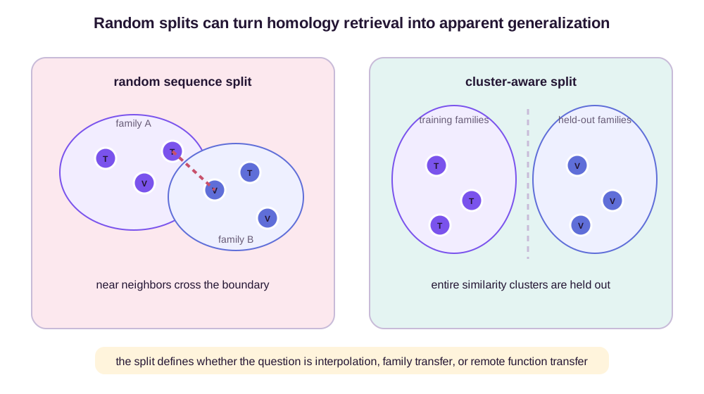
Let \(d(\mathbf a,\mathbf b)\) denote a sequence distance derived from an alignment or search procedure. A cluster-aware split requires

\[\min_{\mathbf a\in\mathcal D_{\mathrm{train}}} d(\mathbf a,\mathbf b) >\delta \qquad \text{for every }\mathbf b\in\mathcal D_{\mathrm{test}}.\]

The threshold \(\delta\), coverage requirement, and clustering algorithm are part of the benchmark. Pairwise identity alone can miss shared domains or local motifs. Structure-based similarity can reveal remote homologs, but filtering on the target structural feature may also alter the problem distribution.

TAPE helped establish task-specific transfer benchmarks rather than treating random sequence splits as sufficient (Rao et al., 2019). The broader principle is to name the intended regime:

• within-family interpolation: predict new variants near characterized homologs;
• family generalization: transfer to a held-out sequence family with related folds or functions;
• function generalization: recognize an activity implemented by a new family or structural solution;
• distribution shift: transfer across organism, assay, environment, or structure source.

These regimes need not rank models in the same order. An MSA may dominate when a deep family is available. A surface encoder may transfer a local interaction pattern across unrelated folds. A large sequence model may be the only practical option when no reliable structure or alignment exists.

One record family under three splits

Consider four records. P0 and P1 share 92% sequence identity; P2 shares 55% with them; Q shares 18% but independently implements the same metal-binding chemistry. Their label dates are 2024, 2020, 2022, and 2025. A fifth record P0-H11Q is an assay variant of P0 measured in the same 2024 campaign.

A row-random split can place P1 and P0-H11Q in training while P0 is in test. The independent unit is nominally a row, but the test record is nearly reconstructible from a homolog and an assay sibling. The estimand is interpolation among related records, even if the table calls it generalization.

At an 80% identity clustering threshold, P0, P1, and P0-H11Q form one group. Holding out that group prevents their crossing, while P2 may remain in training. The test now asks transfer beyond close homologs, but it does not remove remote family or fold similarity. If the threshold were 50%, P2 would join the held-out group and the deployment population would change again.

A temporal cutoff at 2023 trains on labeled P1 and P2 and tests P0, P0-H11Q, and Q when their labels appear. This matches a future-label workflow, but P0 still has close homolog P1 in training. Temporal splitting controls information availability; it does not guarantee family novelty. Conversely, clustering can place a 2020 record in test and no longer represent prospective deployment. A benchmark should name the independent unit, equivalence relation, date policy, and target population because the split name alone specifies none of them.

Family labels are easier than functional mechanisms

Protein families often correlate strongly with function, so high annotation accuracy can arise from locating the correct family neighborhood in embedding space. This is useful when the deployment protein belongs to a known family. It does not establish that the encoder recognized the catalytic mechanism.

Function also exists at several resolutions. Broad Gene Ontology terms, enzyme commission classes, substrate specificity, catalytic rate, binding affinity, and response to a single mutation impose different distinctions. Two homologs can share a fold but differ in substrate. Two unrelated proteins can catalyze similar chemistry. A benchmark that reports only a broad family-correlated label hides both cases.

Concrete evaluation should include counterfactual neighborhoods: close homologs with different functions, distant proteins with convergent functions, mutations around active sites, and matched negatives controlling length, taxonomy, localization, and structure source. Performance should be stratified by similarity to training data rather than summarized only by one area under a curve.

A matched quartet turns that principle into a falsifiable test:

protein	family	identity to family anchor	motif geometry	metal binding
P0	F	100%	intact	yes
P1*	F	92% to P0	H11 rotated away	no
Q0	C	100%	convergently intact	yes
Q1*	C	88% to Q0	donor deleted	no

Assume all four are 58–62 residues, measured in the same assay, expressed in the same host, and supplied from the same structure pipeline. P1* is the close-homolog counterfactual: family remains fixed while mechanism changes. Q0 is the convergent positive: mechanism remains while family changes. Q1* prevents a classifier from treating all of family C as positive.

A pure family rule labels both F proteins positive and both C proteins negative, scoring \(2/4=50\%\). A motif-geometry rule labels P0 and Q0 positive, scoring \(4/4\) on this constructed set. Four records do not estimate population performance, but they diagnose what a larger benchmark must contain. If an embedding succeeds on random family labels and fails this quartet, “captures metal-binding mechanism” is too strong even when aggregate accuracy is high.

What does an embedding actually capture?

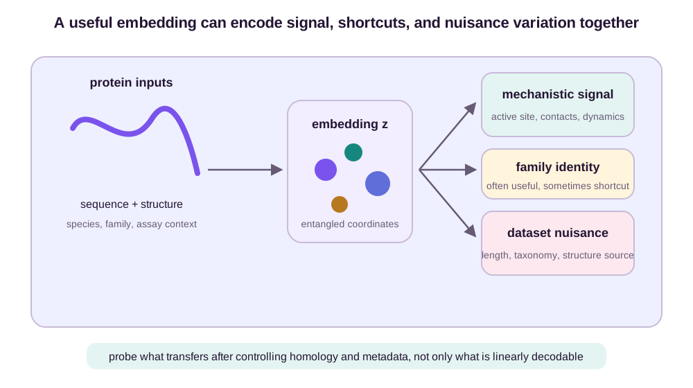
A probing classifier can establish that an attribute is decodable from \(\mathbf z\). It cannot show that the pretrained model uses that attribute, that it is represented independently of a shortcut, or that it will transfer under intervention. High probe accuracy may reflect protein length, taxonomy, subcellular localization, structure confidence, or family membership.

Three tests make embedding claims more precise:

1. Control the probe. Compare against residue composition, length, alignment scores, and frozen random encoders; restrict probe capacity so the probe does not learn the task from scratch.
2. Control the split. Cluster by sequence and, when relevant, structure; group complexes and mutation series; use temporal evaluation for prospective claims.
3. Control the nuisance variables. Match or stratify examples by family, organism, length, experimental method, and predicted-structure confidence.

Retrieval offers another diagnostic. Inspect whether nearest neighbors share only global fold, or also active-site geometry and substrate. Layer-wise analysis can reveal that local syntax, fold, and family information peak at different depths. Fine-tuning can improve task accuracy while destroying a geometry that made the pretrained representation broadly reusable.

The strongest claim is rarely “the embedding contains function.” A defensible claim looks more like this:

Under a stated homology threshold and structure-provenance policy, a fixed representation supports this readout for this functional resolution, and the gain remains after controlling family and metadata baselines.

Four levels of evidence, not one probe score

Start with a nuisance ladder on the same split. Suppose a balanced metal-binding benchmark produces the following hypothetical accuracies:

input and readout	accuracy
majority class	50%
length + amino-acid composition, logistic regression	65%
nearest training-family label	88%
frozen random encoder, linear probe	68%
frozen pretrained embedding, linear probe	91%
frozen pretrained embedding, two-layer MLP	94%

The 91% result establishes linear decodability relative to these baselines. Its incremental gain over nearest family is three points, not 41. The MLP adds another three points, but also has enough capacity to combine weak shortcuts nonlinearly. Probe comparisons need matched regularization, parameter count, training data, and tuning budget; otherwise “the information is nonlinear” can mean only that the larger probe learned more of the task.

Now evaluate the matched quartet. If the linear and MLP probes both score 50% there, the aggregate result remains compatible with family retrieval. If a capacity-restricted geometric probe reaches 4/4, motif geometry is accessible under that controlled readout. The small quartet is diagnostic, while the larger held-out set estimates prevalence-weighted performance. Neither replaces the other.

Downstream use is a stronger and different claim. Fine-tune the encoder for metal binding, then intervene on the motif representation while preserving family features. If zeroing residues 8, 11, and 42 leaves the prediction unchanged but shuffling a family token changes it, the predictor did not use the decoded motif. Conversely, a drop under motif ablation suggests use, although ablation can create off-distribution states.

Intervention stability asks whether matched physical changes produce matched representation changes. Compare P0 with P1*, which preserves family and global fold while rotating one ligand away, and compare P0 with a synonymous metadata change that preserves the molecular object. A mechanistically aligned score should change for the first and remain stable for the second. This test requires a causal intervention or carefully constructed counterfactual; an embedding-space cluster cannot supply it.

The evidentiary ladder is therefore: information is decodable; it is accessible to a restricted probe; a trained predictor actually uses it; and the use persists under interventions that isolate the proposed mechanism. Each step excludes explanations left open by the previous one.

Representation quality is conditional on deployment

Sequence-only models scale to enormous databases and accept proteins without structures. MSAs inject explicit family variation but require homolog search and careful weighting. Residue graphs and frames expose folded geometry but inherit conformation and structure error. Surfaces focus computation on recognition interfaces but discard much of the interior. Multimodal models can share evidence across these views at additional data, compute, and provenance cost.

No representation wins independently of the question. Predicting the effect of one substitution in a well-sampled family, annotating a remote enzyme, finding a binding pocket, and screening an orphan sequence are different inference problems. Their useful neighborhoods, available modalities, and acceptable leakage risks differ.

A deployment claim should therefore freeze an interface contract. For an orphan-protein annotation system, that contract might be:

• input sequence is available at decision time, but no minimum MSA depth is assumed;
• predicted structure may be used only from a named model and database snapshot predating the decision;
• the readout predicts one declared metal-binding assay, not broad family membership;
• train/test dependence is controlled at 50% sequence identity and by mutation-series grouping;
• a linear probe and a fixed two-layer probe are reported beside composition and nearest-family baselines;
• the matched quartet tests close-homolog negatives and convergent positives;
• calibration and abstention are evaluated separately for deep-MSA and orphan strata;
• prospective mutations of the coordinating motif test whether the decision changes in the expected direction.

Under this contract, 91% linear-probe accuracy supports decodability on the stated population. It does not prove the fine-tuned model uses the motif. Success on P0/P1* and Q0/Q1* strengthens the mechanism claim. Prospective stability under motif interventions strengthens it again. If the system instead deploys within a known family, the nearest-family baseline may be the appropriate competitor and MSA evidence may be entirely legitimate. The scientific claim changes with the deployment regime, not only with the headline accuracy.

The central discipline is to keep three boundaries visible: what entered the encoder, what the pretraining loss rewarded, and what similarity remained across the evaluation split. Once those boundaries are explicit, protein embeddings become easier to interpret. They are compressed views of particular datasets under particular objectives—not universal coordinates of biological meaning, but often powerful representations when their preserved information matches the deployment problem.

References

1. Rives, A. et al. (2021). Biological Structure and Function Emerge from Scaling Unsupervised Learning to 250 Million Protein Sequences. Proceedings of the National Academy of Sciences. ↩
2. Rao, R. M. et al. (2021). MSA Transformer. ICML. ↩
3. Jing, B., Eismann, S., Suriana, P., Townshend, R. J. L., & Dror, R. O. (2021). Learning from Protein Structure with Geometric Vector Perceptrons. ICLR. ↩
4. Zhang, Z. et al. (2023). Protein Representation Learning by Geometric Structure Pretraining. ICLR. ↩
5. Gainza, P. et al. (2020). Deciphering Interaction Fingerprints from Protein Molecular Surfaces Using Geometric Deep Learning. Nature Methods. ↩
6. Su, J., Han, C., Zhou, Y., Shan, J., Zhou, X., & Yuan, F. (2024). SaProt: Protein Language Modeling with Structure-Aware Vocabulary. ICLR. ↩
7. Rao, R. et al. (2019). Evaluating Protein Transfer Learning with TAPE. NeurIPS. ↩

---

Figure provenance. All four protrep_ diagrams are original SVG illustrations generated by scripts/generate_protrep_figures.py. They synthesize standard representation, pretraining, and evaluation concepts described in the cited primary literature; no third-party artwork is reproduced.