Machine Learning Meets Quantum Chemistry

Adapted from my 2025 Machine Learning for Molecules lectures. Building on Quantum Chemistry and DFT, this article asks what a learned model actually approximates—wavefunction, density, Hamiltonian, energy surface, property, or correction—and how its error propagates through the solver or estimator that consumes it.

Quantum chemistry is expensive for a structural reason. The electronic state of \(N_e\) electrons is not a function of one point in three-dimensional space; it is a function over all electron coordinates at once. Machine learning can avoid, accelerate, or reparameterize parts of that computation, but these interventions are not interchangeable.

A neural wavefunction still solves a variational many-electron problem for each system. A learned exchange-correlation functional remains inside a self-consistent density-functional calculation. A Hamiltonian or density surrogate predicts an electronic object directly. An interatomic potential skips the electronic variables and learns the Born–Oppenheimer energy surface. A property model goes further and predicts one observable.

Moving down this ladder usually makes inference cheaper. It also narrows what can be reused and weakens the connection to first-principles constraints. The central question is therefore not whether machine learning “solves quantum chemistry,” but which quantum-chemical map it replaces, under which fidelity and domain, and what computation remains after the network returns.

The many-electron problem creates the bottleneck

Under the Born–Oppenheimer approximation, nuclear positions \(\mathbf{R}=(\mathbf{R}_1,\ldots,\mathbf{R}_{N_n})\) are fixed while the electronic problem is solved:

\[\widehat H_{\mathbf R}\,\Psi(\mathbf r_1,\ldots,\mathbf r_{N_e}) = E(\mathbf R)\,\Psi(\mathbf r_1,\ldots,\mathbf r_{N_e}).\]

In atomic units, the electronic Hamiltonian contains

\[\widehat H_{\mathbf R} = -\frac12\sum_{i=1}^{N_e}\nabla_i^2 -\sum_{i,A}\frac{Z_A}{\lVert\mathbf r_i-\mathbf R_A\rVert} +\sum_{i<j}\frac{1}{\lVert\mathbf r_i-\mathbf r_j\rVert} +E_{\mathrm{nn}}(\mathbf R).\]

The first term is electronic kinetic energy, the second is electron–nuclear attraction, the third is electron–electron repulsion, and the last is nuclear repulsion. The electron–electron term prevents the equation from separating into independent one-electron problems.

The wavefunction lives on a \(3N_e\)-dimensional configuration space and must be antisymmetric under exchange of same-spin electrons:

\[\Psi(\ldots,\mathbf r_i,\ldots,\mathbf r_j,\ldots) = -\Psi(\ldots,\mathbf r_j,\ldots,\mathbf r_i,\ldots).\]

This sign change is not optional structure that more data can teach reliably. It encodes fermionic statistics and creates nodes where the wavefunction vanishes. Classical approximations trade accuracy for tractability: Hartree–Fock uses a mean-field Slater determinant, post-Hartree–Fock methods recover electron correlation at rapidly increasing cost, and density functional theory replaces the high-dimensional wavefunction with the three-dimensional electron density.

Common formal scaling labels—roughly cubic for conventional Kohn–Sham DFT, quartic for Hartree–Fock, and seventh power for canonical CCSD(T)—are useful warnings, not runtime laws. Basis size, sparsity, system geometry, implementation, memory, convergence, and desired precision can dominate the observed cost.

Machine learning can target different objects

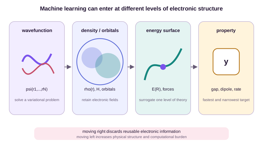
These targets define distinct method boundaries:

Learned object	Model output	Computation that remains	Typical transfer boundary
Wavefunction	\(\Psi_\theta(\mathbf r;\mathbf R)\)	Monte Carlo sampling and variational optimization	New system often needs optimization
Exchange-correlation functional	\(E_{\mathrm{xc},\theta}[\rho]\)	Functional differentiation and self-consistent Kohn–Sham solve	Densities and chemistry covered by training
Hamiltonian / density	Matrix elements or \(\rho(\mathbf r)\)	Diagonalization, observables, or validation	Basis, elements, geometries, level of theory
Energy surface	\(E_\theta(\mathbf R)\) and derivatives	Geometry optimization or dynamics	Composition and configuration coverage
Property	One or several observables	Usually only a forward pass	Exact label definition and data domain
Correction	\(\Delta_\theta=Y_{\mathrm{high}}-Y_{\mathrm{low}}\)	Low-fidelity baseline plus correction	Stability of the residual across domain

A model at one row should not inherit the claims of another. Predicting energies accurately does not imply accurate electron density. Predicting a Hamiltonian matrix does not remove the cost of solving its eigenproblem. A neural wavefunction is not an amortized property predictor if it must be reoptimized for each molecular geometry.

Neural wavefunctions keep the variational problem

For any normalized trial wavefunction \(\Psi_\theta\), the variational principle gives

\[E_\theta = \frac{\langle\Psi_\theta\vert\widehat H\vert\Psi_\theta\rangle} {\langle\Psi_\theta\vert\Psi_\theta\rangle} \ge E_0,\]

where \(E_0\) is the exact ground-state energy in the chosen Hamiltonian. This inequality gives neural wavefunctions a physical training objective and an interpretable direction of improvement.

Variational Monte Carlo rewrites the energy as an expectation under

\[p_\theta(\mathbf r) = \frac{\lvert\Psi_\theta(\mathbf r)\rvert^2} {\int\lvert\Psi_\theta(\mathbf r')\rvert^2d\mathbf r'}.\]

Define the local energy

\[E_{\mathrm L}(\mathbf r) = \frac{\widehat H\Psi_\theta(\mathbf r)} {\Psi_\theta(\mathbf r)}.\]

Then

\[E_\theta = \mathbb E_{\mathbf r\sim p_\theta} \left[E_{\mathrm L}(\mathbf r)\right].\]

The network is optimized using electron configurations sampled from its own squared amplitude. A perfect eigenstate has constant local energy wherever its probability is nonzero, so local-energy variance is also a useful diagnostic.

A two-level state exposes variational and sampling error

Take a Hamiltonian with orthonormal eigenstates \(\lvert0\rangle,\lvert1\rangle\) and energies 0 and 2:

\[\widehat H =0\lvert0\rangle\langle0\rvert +2\lvert1\rangle\langle1\rvert.\]

Choose a normalized trial state

\[\lvert\Psi_\theta\rangle =\sqrt{0.9}\lvert0\rangle +\sqrt{0.1}\lvert1\rangle.\]

Its exact variational energy is

\[E_\theta=0.9(0)+0.1(2)=0.2\geq E_0=0.\]

If Monte Carlo configurations are the two basis states, the local energy is 0 with probability 0.9 and 2 with probability 0.1. Its variance is

\[\begin{aligned} \operatorname{Var}(E_{\mathrm L}) &=0.9(0-0.2)^2+0.1(2-0.2)^2\\ &=0.36. \end{aligned}\]

The trial state is close in overlap to the ground state, yet rare excited-state samples dominate its estimator variance. For 100 independent samples, the energy standard error is

\[\operatorname{SE}(\widehat E) =\sqrt{0.36/100}=0.06.\]

VMC samples usually come from a Markov chain rather than independently. Suppose the normalized energy autocorrelation is \(\rho_\ell=0.8^\ell\) at lag \(\ell\). The integrated autocorrelation time is

\[\tau_{\mathrm{int}} =1+2\sum_{\ell=1}^{\infty}\rho_\ell =1+2\frac{0.8}{1-0.8} =9.\]

The 100 stored values then represent only about \(100/9=11.1\) independent samples, raising the standard error to

\[\sqrt{0.36/11.1}\approx0.18.\]

The variational principle constrains the exact expectation \(E_\theta\), not every finite Monte Carlo estimate. An estimate centered at 0.2 with standard error 0.18 can fluctuate below zero. More samples reduce estimator error; they do not reduce the ansatz error of 0.2. Changing the trial state reduces ansatz error and often local-energy variance, but may also change Markov-chain mixing. These three quantities should be reported separately.

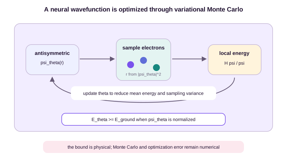
FermiNet builds antisymmetry through determinants of learned, many-electron-dependent orbitals and demonstrated highly accurate first-principles energies (Pfau et al., 2020). Its neural network is not merely regressing against energy labels: the Hamiltonian supplies the objective. This avoids a precomputed energy dataset, but it does not make the calculation free. Sampling high-dimensional electron configurations, evaluating derivatives in the kinetic-energy operator, and optimizing a noisy nonconvex objective remain expensive.

The variational bound also needs careful interpretation. It holds for the expectation represented by the trial state and Hamiltonian. A noisy Monte Carlo estimate can fluctuate below a reference value. Comparisons can also be limited by pseudopotentials, basis or boundary choices, relativistic effects, and imperfect reference energies. “Lower is better” is meaningful only when these choices match.

Density functional theory moves the unknown into a functional

The Hohenberg–Kohn result establishes that the ground-state density determines the external potential, and therefore ground-state observables, under its assumptions (Hohenberg & Kohn, 1964). Kohn–Sham DFT writes the energy schematically as

\[E[\rho] = T_s[\rho] +E_{\mathrm H}[\rho] +\int v_{\mathrm{ext}}(\mathbf r)\rho(\mathbf r)d\mathbf r +E_{\mathrm{xc}}[\rho] +E_{\mathrm{nn}}.\]

The noninteracting kinetic energy \(T_s\) is evaluated through Kohn–Sham orbitals, the Hartree term \(E_{\mathrm H}\) is classical Coulomb repulsion, and the exchange-correlation functional \(E_{\mathrm{xc}}\) absorbs the remaining many-body effects.

Learning \(E_{\mathrm{xc},\theta}[\rho]\) is attractive because one learned object can improve many systems and observables while preserving the Kohn–Sham machinery. But the functional is used through its derivative

\[v_{\mathrm{xc},\theta}(\mathbf r) = \frac{\delta E_{\mathrm{xc},\theta}[\rho]} {\delta\rho(\mathbf r)}.\]

The derivative enters the effective Hamiltonian, which produces new orbitals and a new density. The model therefore participates in a fixed-point iteration:

\[\rho_k \longrightarrow \widehat H_{\mathrm{KS}}[\rho_k] \longrightarrow \{\phi_i^{(k)}\} \longrightarrow \rho_{k+1}.\]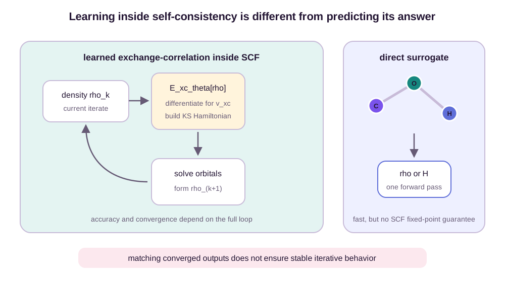

This explains why fitting energies on converged reference densities is not enough. The learned functional will encounter its own intermediate densities at deployment. Its derivatives must be sensible, the SCF iteration must converge, and exact constraints outside the energy training set may matter. DM21 illustrates how incorporating fractional-electron constraints can address known functional failures rather than relying only on benchmark fitting (Kirkpatrick et al., 2021).

The learned derivative controls fixed-point stability

A scalar fixed point isolates what the functional derivative does to SCF. Let \(n_k\) denote one density mode and suppose the reference SCF map is

\[n_{k+1}=F(n_k)=0.4+0.5n_k.\]

Its fixed point is \(n^\star=0.4/(1-0.5)=0.8\). Because \(F'(n)=0.5\), perturbations contract by a factor of two each iteration. Starting from \(n_0=0\) gives \(0.4,0.6,0.7,0.75,\ldots\).

Now suppose a learned functional preserves the same fixed point but changes the response derivative:

\[\widehat F(n)=1.76-1.2n.\]

Indeed, \(\widehat F(0.8)=0.8\), so evaluating the model only at the converged density would not expose the problem. But \(\widehat F'(n)=-1.2\) has magnitude above one. Starting from zero produces

\[1.76,\;-0.352,\;2.1824,\;-0.8589,\;\ldots,\]

an oscillation with growing amplitude. The fixed point is correct and the iteration is unusable.

Linear mixing replaces the raw update by

\[n_{k+1}=(1-\eta)n_k+\eta\widehat F(n_k).\]

Its derivative is \(1-\eta+\eta(-1.2)=1-2.2\eta\). With \(\eta=0.5\), the mixed map is \(n_{k+1}=0.88-0.1n_k\) and the sequence becomes

\[0.88,\;0.792,\;0.8008,\;0.79992,\;\ldots.\]

Mixing restores contraction for this mode without changing the fixed point. It does not make an arbitrary learned functional safe: several density modes can have different eigenvalues, and no single scalar \(\eta\) need condition all of them well. Energy fit on converged densities constrains function values. SCF stability depends on functional derivatives and the Jacobian of the complete density-to-density map.

There is a crucial distinction between a model that learns a functional and one that learns energies from density descriptors. Only the former is intended to be differentiated and used self-consistently. The latter may be an accurate correction at a fixed density without defining a stable Kohn–Sham procedure.

Density, orbitals, and Hamiltonians preserve reusable structure

Instead of learning the functional, a model can predict the output of an electronic-structure calculation.

A density model maps nuclear geometry and a query point to

\[\rho_\theta(\mathbf r\mid\mathbf R,\mathbf Z).\]

The basic constraints include nonnegativity and electron count,

\[\rho_\theta(\mathbf r)\ge0, \qquad \int\rho_\theta(\mathbf r)d\mathbf r=N_e.\]

DeepDFT treats query locations as graph nodes and predicts charge density around molecules and materials (Jørgensen & Bhowmik, 2022). Pointwise prediction is flexible but expensive on a dense grid. Predicting coefficients in atom-centered basis functions or using a neural operator amortizes spatial evaluation, at the cost of committing to a basis and resolution.

A Hamiltonian model instead predicts matrix elements in a chosen orbital basis:

\[H_{\mu\nu,\theta}(\mathbf R) \approx \langle\chi_\mu\vert\widehat H_{\mathrm{KS}}\vert\chi_\nu\rangle.\]

These blocks transform nontrivially when the molecule rotates because atomic orbitals carry angular momentum. Equivariant architectures such as QHNet encode that transformation law directly (Yu et al., 2023). The predicted matrix can initialize SCF, produce orbitals after diagonalization, or support downstream electronic observables.

But a small matrix-element MAE is not automatically a small orbital or energy error. Near degeneracies, small perturbations can rotate eigenvectors strongly. A Hamiltonian tied to one basis set, pseudopotential, and functional is not a basis-independent electronic truth. Evaluation should therefore include derived eigenvalues, densities, forces, SCF iterations, and target observables—not only entrywise error.

A small matrix error can rotate a near-degenerate orbital

Consider the nearly degenerate reference Hamiltonian

\[\mathbf H =\begin{bmatrix}-0.01&0\\0&0.01\end{bmatrix}.\]

Its eigenvalues are \(-0.01\) and \(0.01\), and its eigenvectors are the two basis orbitals. Suppose the learned model makes only an off-diagonal error of 0.01:

\[\widehat{\mathbf H} =\begin{bmatrix}-0.01&0.01\\0.01&0.01\end{bmatrix}.\]

Averaged over all four matrix entries, the absolute error is only 0.005. Diagonalization gives

\[\widehat\varepsilon_\pm =\pm\sqrt{0.01^2+0.01^2} =\pm0.01414.\]

The predicted gap is 0.02828 rather than 0.02, a 41.4% error. Up to the sign convention for eigenvectors, the magnitude of the orbital rotation satisfies

\[\tan(2\lvert\theta\rvert)=\frac{2(0.01)}{0.01-(-0.01)}=1, \qquad \lvert\theta\rvert=22.5^\circ.\]

The same 0.01 off-diagonal perturbation would barely rotate orbitals separated by an energy gap of 1. Near degeneracy makes the eigenspace ill-conditioned. Entrywise MAE does not encode this denominator, so Hamiltonian evaluation should stratify by spectral gaps and test subspaces, eigenvalues, densities, and observables after diagonalization.

Density constraints do not determine density observables

A two-point grid gives an equally small witness for density prediction. Put grid locations at \(x=-1\) and \(x=+1\) with unit quadrature weights. A one-electron reference density

\[\boldsymbol\rho=(0.6,0.4)\]

has electron count 1 and dipole

\[\mu=\sum_jx_j\rho_j=-0.6+0.4=-0.2.\]

The prediction \((0.55,0.55)\) is nonnegative and has pointwise MAE 0.10, but integrates to 1.10 electrons. Renormalizing it gives \((0.5,0.5)\) and repairs electron count while leaving dipole 0, an error of 0.2. Conversely, \((0.7,0.3)\) has exactly the correct normalization but dipole \(-0.4\). Positivity and normalization are necessary constraints. They do not certify multipoles, electrostatic potentials, response, or energy functionals evaluated on the density.

Surrogate potentials and properties skip electronic variables

For fixed nuclear charges, the electronic calculation defines a Born–Oppenheimer energy surface \(E(\mathbf R)\). A machine-learned interatomic potential approximates this map and obtains forces by differentiation:

\[\mathbf F_A = -\nabla_{\mathbf R_A}E_\theta(\mathbf R).\]

This is the right boundary for long molecular-dynamics trajectories when electronic densities are unnecessary. It can provide orders-of-magnitude faster force evaluations after training. It does not discover new electronic states beyond its reference data, and it inherits the level of theory used for the labels. The companion post on equivariant Transformers and machine-learned potentials develops the conservation, cutoff, and scaling requirements.

A direct property model is narrower still:

\[y_\theta=f_\theta(\mathbf Z,\mathbf R)\]

for an orbital gap, dipole, excitation energy, or reaction barrier. Such a model can be extremely efficient and may need fewer outputs than a universal potential. Its label must be defined precisely: method, basis, charge, spin state, geometry, environment, and thermodynamic corrections are part of the target. A model cannot be “DFT accurate” when different functionals disagree materially and the reference functional is unnamed.

The two outputs support different contracts. An energy surface supplies a scalar over a geometry domain and, when differentiated, conservative forces. That contract supports geometry optimization or dynamics only after smoothness, coverage, and numerical integration are validated in the companion chapters. A property head supplies one labeled functional of geometry. A dipole head need not define an energy, a density, or forces; an excitation-energy head need not order ground-state conformers correctly.

Narrowness can be an advantage. If a screen needs one vertical excitation at fixed geometry, predicting a full Hamiltonian and diagonalizing it may be wasted computation. Narrowness also prevents reuse: changing from vertical to adiabatic excitation introduces geometry relaxation, and adding solvent or temperature changes the target. The output contract must list the geometry protocol and physical conditions rather than hiding them behind the property name.

Learned corrections exploit a cheaper baseline

Often the most data-efficient target is a discrepancy:

\[\Delta(\mathbf x) = Y_{\mathrm{high}}(\mathbf x) -Y_{\mathrm{low}}(\mathbf x),\]

so that

\[Y_{\mathrm{pred}}(\mathbf x) = Y_{\mathrm{low}}(\mathbf x) +\Delta_\theta(\mathbf x).\]

If the inexpensive method already captures most variation, the residual can be smoother and smaller than the full high-fidelity target. Delta machine learning demonstrated this strategy across chemical space (Ramakrishnan et al., 2015).

The benefit depends on correlation, not merely on the baseline being cheap. Consider two low-fidelity methods with the same MAE. One makes a nearly constant systematic error; its residual is easy to learn. The other has geometry-dependent sign changes; its residual may be as difficult as the original target. Baseline cost remains at inference, and any catastrophic baseline failure passes into the corrected prediction unless the model learns that regime.

Multi-fidelity training also creates bookkeeping risks. Geometries must correspond across methods. Atomization energies, total energies, and thermal corrections cannot be mixed casually. A reference computed on a geometry optimized at another level includes both electronic and geometry discrepancies.

Equal baseline MAE can hide opposite residual difficulty

Take four high-fidelity values

\[\mathbf Y_{\mathrm{high}}=(10,20,30,40).\]

Baseline A predicts \((8,18,28,38)\). Baseline B predicts \((8,22,28,42)\). Both have MAE 2, but their correction targets are

\[\boldsymbol\Delta_A=(2,2,2,2), \qquad \boldsymbol\Delta_B=(2,-2,2,-2).\]

Baseline A needs only an intercept to become exact. Baseline B needs a feature that distinguishes the alternating cases; without it, the best constant correction is zero and the MAE remains 2. The baselines have equal standalone accuracy and unequal value for delta learning because residual structure, not baseline MAE alone, determines learnability.

The corrected error decomposes as

\[Y_{\mathrm{pred}}-Y_{\mathrm{high}} =\Delta_\theta-\Delta.\]

The baseline cancels algebraically only when it is evaluated under the same definition at inference. If baseline B fails to converge on one geometry, changes electronic state, or uses a mismatched optimized structure, the intended residual may no longer be defined. A fallback policy and baseline failure rate belong in both accuracy and cost reports.

Transfer across chemical space is a coverage problem

Electronic-structure models face several axes of extrapolation at once:

• new elements and oxidation states;
• larger electron counts and molecular sizes;
• bond breaking, stretched geometries, and transition states;
• charge and spin multiplicity;
• excited states and near degeneracies;
• intermolecular interactions and long-range charge transfer;
• molecules versus periodic materials;
• basis sets, pseudopotentials, and reference methods.

Pretraining can amortize representations or initialize wavefunctions and Hamiltonians across related systems. It does not remove these axes. A model trained on neutral equilibrium organic molecules may interpolate impressively while failing on an ion, radical, or dissociation curve.

Size extensivity and locality help some outputs. Energy may be decomposed approximately into local contributions for insulating systems, enabling transfer to larger structures. Orbitals, response properties, charged excitations, and metallic systems can remain globally coupled. The architecture should not impose locality more aggressively than the physics allows.

Dissociation and charge reveal missing inputs

Suppose a local model was trained on neutral diatomics near equilibrium and uses cutoff \(r_c=5\) bohr. Beyond the cutoff, its two atomic environments no longer communicate, so its predicted interaction approaches a constant. For an oppositely charged dissociation channel, however, the asymptotic interaction contains

\[E(R)-E(\infty)=-\frac{1}{R}.\]

At \(R=10\) bohr, omitting this tail creates an error of 0.1 hartree, about 2.72 eV. At 20 bohr the error is still 1.36 eV. More neutral near-equilibrium data cannot teach a dependence that the cutoff removes and the training domain never visits.

Charge can produce an even simpler collision. If a model input contains only nuclear species and geometry, the same geometry for a neutral molecule and its cation is identical to the network. Their electron counts, densities, Hamiltonians, and energies differ. A deterministic predictor must return the same output for both unless total charge or an equivalent electronic-state descriptor is supplied. This is not ordinary covariate shift; the requested map is not a function of the provided input.

OOD evaluation should therefore name the changed axis. Stretched geometries test configurational coverage. New charge or spin tests missing state variables and their representation. New elements test learned chemical embeddings. A larger molecule can test size extrapolation while remaining locally familiar. Collapsing these into one aggregate “OOD MAE” hides which intervention could fix the failure.

Data fidelity is part of the target

Quantum-chemical labels are computed, but they are not ground truth in an absolute sense. They depend on a hierarchy of choices:

\[\text{Hamiltonian} \rightarrow \text{relativistic/pseudopotential approximation} \rightarrow \text{electronic method} \rightarrow \text{basis and thresholds} \rightarrow \text{numerical convergence}.\]

A model can reproduce its labels more accurately than those labels reproduce experiment. This is not paradoxical; it is emulation. Reported error against CCSD(T) measures imitation of that protocol, not error against the exact Schrödinger solution. Experimental comparison adds nuclear quantum effects, temperature, environment, and measurement uncertainty.

Physical constraints can prevent some failures:

• antisymmetry for fermionic wavefunctions;
• normalization and cusp/asymptotic behavior;
• nonnegative density with correct electron count;
• Hermitian, rotation-covariant Hamiltonian matrices;
• invariant extensive energy and conservative forces;
• exact or known limiting constraints for density functionals.

Constraints narrow the hypothesis class but do not certify chemical accuracy. An antisymmetric wavefunction can still have a poor nodal surface. A normalized density can be spatially wrong. A conservative potential can conserve the wrong energy surface.

Fidelity can reverse the scientific decision

Consider three candidate geometries with low-fidelity energies

\[Y_{\mathrm{low}}(A,B,C)=(-10,-9,-8).\]

Lower is preferred, so the baseline ranks \(A\prec B\prec C\). Suppose high-level corrections are \((+3,-1,-4)\). Then

\[Y_{\mathrm{high}}(A,B,C)=(-7,-10,-12),\]

and the ranking reverses to \(C\prec B\prec A\). A surrogate with 0.1 error against the low-fidelity labels would emulate their ranking accurately and still choose the wrong high-fidelity candidate. “Chemical accuracy” needs a named reference and a decision margin; an absolute error smaller than typical energy scales does not guarantee preserved ranking when candidates are close or fidelity corrections are structured.

Experimental ranking adds another layer. Zero-temperature electronic energies omit thermal and entropic corrections; solution measurements add environment and protocol. Fidelity is not one vertical axis with experiment at a universally comparable top. Each label denotes a particular physical quantity, and candidate ranking is valid only for the quantity that drives the decision.

Accuracy-versus-cost claims need a denominator

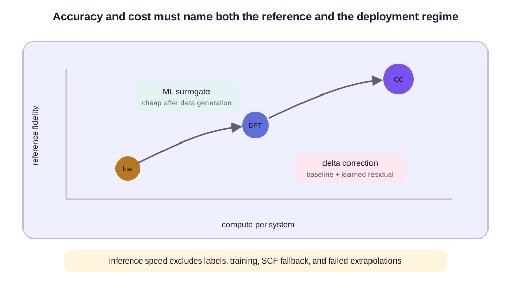
“A thousand times faster than DFT” can describe several different comparisons. Is the baseline one SCF energy, a geometry optimization, or an entire trajectory? Does ML timing include neighbor construction, force derivatives, diagonalization, and uncertainty checks? Is the reference running on CPU while the network uses a GPU? Is data generation and training amortized over ten predictions or ten million?

Accuracy needs the same specificity. Report energy per atom and total energy when extensivity matters. Report forces if dynamics are claimed. Test relative conformer energies, reaction barriers, density integrals, eigenvalues, and SCF convergence according to the use case. Stratify by system size and chemical novelty. Compare at matched geometries and units.

A useful cost statement has the form:

For this chemical domain, reference protocol, hardware, batch size, and required outputs, the trained model reaches this error distribution at this wall-clock and memory cost, including the remaining numerical steps.

That sentence is less dramatic than “quantum accuracy at ML speed,” but it is scientifically transferable.

Break-even depends on everything that remains

Let one matched-output reference calculation cost 100 GPU-hours. Suppose generating the training labels costs 10,000 GPU-hours and model training costs another 2,000. A nominal forward pass costs 0.001 GPU-hours, but the promised output also requires 0.020 GPU-hours of diagonalization or remaining solver work and 0.002 GPU-hours of uncertainty checks. If 5% of queries fall back to the reference, the expected deployed cost is

\[C_{\mathrm{ML}} =0.001+0.020+0.002+0.05(100) =5.023\ \text{GPU-hours/query}.\]

For \(Q\) production queries, the learned route costs

\[C_{\mathrm{total}}(Q)=12{,}000+5.023Q,\]

while direct reference computation costs \(100Q\). Break-even occurs at

\[Q_\star =\frac{12{,}000}{100-5.023} \approx126.3.\]

The 127th query is the first one beyond this simplified break-even. If deployment needs only 100 queries, the learned route costs more in total despite a forward pass that is 100,000 times cheaper than the reference. If the fallback rate rises from 5% to 50%, expected inference becomes 50.023 GPU-hours and break-even rises to about 240 queries.

The numerator should count only reference data and training dedicated to the claimed use, or explicitly state how a reused foundation model amortizes them across tasks. The denominator requires matched hardware, batch size, precision, and output. Timing an energy-only network on a GPU against a CPU reference that returns energy, forces, stress, and orbitals does not compare the same map. Hamiltonian prediction must include diagonalization if eigenvalues are claimed; delta learning must include its baseline; a wavefunction method must include system-specific optimization and sampling.

Memory, latency, and failure handling can dominate wall-clock averages. A large batched model may have excellent throughput and poor single-geometry latency. A rare fallback can serialize an otherwise fast pipeline. The cost claim should therefore report total resource, latency distribution, remaining solver iterations, failure denominator, and the number of deployments over which training is amortized.

Where machine learning genuinely changes the calculation

Machine learning contributes in three distinct ways. It can amortize a repeated map, as in property, energy, density, or Hamiltonian surrogates. It can improve an approximation within a physical solver, as in learned exchange-correlation functionals. Or it can enlarge the variational ansatz, as in neural wavefunctions.

Each route has a different source of truth. Supervised surrogates are bounded by data coverage and fidelity. Learned functionals are judged by self-consistent behavior and physical constraints, not only label fit. Neural wavefunctions retain a first-principles variational objective but pay system-specific sampling and optimization cost.

The most useful boundary is often not the deepest one. If a molecular-dynamics trajectory needs only energies and forces, predicting a wavefunction is unnecessarily expensive. If many electronic observables are needed, a one-property model is too narrow. If extrapolation into new correlation regimes matters, a direct surrogate may be risky even when its interpolation error is tiny.

The worked examples turn that choice into an interface contract:

Learned object	Downstream operation	Perturbation-sensitive diagnostic	Cost that remains
Wavefunction	Monte Carlo expectation and optimization	Local-energy variance, autocorrelation, variational energy	Sampling and usually system-specific optimization
Functional	Functional derivative and SCF fixed point	Density-response Jacobian, convergence, final energy and density	Hamiltonian construction, diagonalization, SCF iterations
Hamiltonian	Generalized eigensolve or SCF initialization	Gap-stratified eigenvalues and orbital subspaces	Diagonalization and any remaining self-consistency
Density	Quadrature and observable functionals	Electron count, multipoles, energies, response	Grid or basis evaluation and downstream functional
Potential	Derivatives, optimizer, or trajectory	Forces, smoothness, distributional and observable tests	Geometry optimization or integration
Property	Usually direct decision	Label-specific calibration and ranking	Little solver work, little reuse outside that property
Correction	Baseline plus learned residual	Residual structure, baseline failures, corrected ranking	Every baseline calculation and fallback

No row is uniformly best. Moving downward usually amortizes more computation but commits earlier to an output. Moving upward preserves reusable electronic structure but leaves more numerical work and more ways for small learned errors to be amplified. The appropriate validation follows the downstream operation: sample a wavefunction, iterate a functional, diagonalize a Hamiltonian, integrate a density, differentiate a potential, or act on a property.

Machine learning meets quantum chemistry productively when it makes that boundary explicit. The network should replace exactly the part whose repeated cost dominates, preserve the constraints required downstream, and expose when the system has left the chemical and numerical regime represented by its training or variational family.

References

1. Pfau, D., Spencer, J. S., Matthews, A. G. D. G., & Foulkes, W. M. C. (2020). Ab Initio Solution of the Many-Electron Schrödinger Equation with Deep Neural Networks. Physical Review Research. ↩
2. Hohenberg, P., & Kohn, W. (1964). Inhomogeneous Electron Gas. Physical Review. ↩
3. Kirkpatrick, J. et al. (2021). Pushing the Frontiers of Density Functionals by Solving the Fractional Electron Problem. Science. ↩
4. Jørgensen, P. B., & Bhowmik, A. (2022). DeepDFT: Neural Message Passing Network for Accurate Charge Density Prediction. Frontiers in Materials. ↩
5. Yu, H., Xu, Z., Qian, X., Qian, X., & Ji, S. (2023). Efficient and Equivariant Graph Networks for Predicting Quantum Hamiltonian. ICML. ↩
6. Ramakrishnan, R., Dral, P. O., Rupp, M., & von Lilienfeld, O. A. (2015). Big Data Meets Quantum Chemistry Approximations: The Delta-Machine Learning Approach. Journal of Chemical Theory and Computation. ↩

---

Figure provenance. All four mlqc_ diagrams are original SVG illustrations generated by scripts/generate_mlqc_figures.py. They synthesize standard electronic-structure and machine-learning workflows described in the cited primary literature; no third-party artwork is reproduced.