Graph Neural Networks as Learnable Message Passing

Adapted from my 2025 Machine Learning for Molecules and Geometric Deep Learning lectures. The focus is the symmetry constraint that makes a neural network a graph network, the familiar architectures that follow from it, and the limitations that remain.

An image is an array before it enters a neural network. Its row and column indices tell us which pixels are adjacent, and the same small filter can be applied at every location. A graph gives us no such coordinate system. It gives us entities, relations, and an arbitrary choice of indices used to store them.

That missing coordinate system is not an inconvenience to work around. It determines the architecture. A graph neural network must produce the same graph prediction after we rename every node. For a node-wise prediction, renaming the input nodes must rename the outputs in exactly the same way. Message passing is the simplest learnable computation that satisfies these requirements while respecting the graph’s sparse relations.

The same abstraction contains graph convolutional networks (GCNs), GraphSAGE, graph attention networks (GATs), and graph isomorphism networks (GINs). Their differences matter, but they are variations on three decisions: what a neighbor sends, how a node combines an unordered collection of messages, and how the node mixes that result with its current state. Graph Transformers loosen the locality constraint, then face a complementary problem: once every node can communicate with every other node, the model must be told which pairs were connected in the original graph.

A graph has relations but no canonical order

Let a graph be \(G=(V,E)\), where \(V\) is a set of nodes and \(E\) is a set of edges. Suppose there are \(n\) nodes, each with a feature vector. We store the features in a matrix

\[\mathbf{X}\in\mathbb{R}^{n\times d},\]

and the edges in an adjacency matrix

\[\mathbf{A}\in\{0,1\}^{n\times n}.\]

The first row of \(\mathbf{X}\) belongs to the node assigned index 1, but that assignment carries no meaning. In a molecular graph, switching the stored indices of two carbon atoms does not create a new molecule. In a citation graph, reordering the papers in a database does not change who cites whom.

The contrast with a fixed grid is shown below. A pixel grid has named offsets such as one step left or one step up. A graph only specifies which nodes are related.

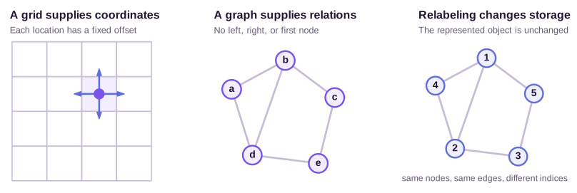
We can state the required symmetry with a permutation matrix \(\mathbf{P}\). Multiplying \(\mathbf{X}\) by \(\mathbf{P}\) reorders its rows. The same relabeling changes the adjacency matrix to

\[\mathbf{A}'=\mathbf{P}\mathbf{A}\mathbf{P}^{\mathsf T}.\]

A node-level model \(F\) should be permutation equivariant:

\[F(\mathbf{P}\mathbf{X},\mathbf{P}\mathbf{A}\mathbf{P}^{\mathsf T}) =\mathbf{P}F(\mathbf{X},\mathbf{A}).\]

The output changes because the output rows must follow the renamed nodes. A graph-level model \(f\) should instead be permutation invariant:

\[f(\mathbf{P}\mathbf{X},\mathbf{P}\mathbf{A}\mathbf{P}^{\mathsf T}) =f(\mathbf{X},\mathbf{A}).\]

These equations do not say that every node is interchangeable. Node features and connectivity can make two nodes structurally different. They say that the numerical index assigned to a node cannot affect the answer.

Message passing is a learnable set function

A message-passing layer updates each node from its current state and the states of its neighbors. Let \(\mathbf{h}_v^{(\ell)}\) denote the hidden state of node \(v\) after layer \(\ell\), and let \(\mathbf{e}_{uv}\) denote an optional feature on the edge from \(u\) to \(v\). One layer first computes a message

\[\mathbf{m}_{u\to v}^{(\ell)} =M^{(\ell)}\!\left( \mathbf{h}_u^{(\ell-1)}, \mathbf{h}_v^{(\ell-1)}, \mathbf{e}_{uv} \right),\]

then combines all incoming messages and updates the receiver:

\[\mathbf{a}_v^{(\ell)} =\operatorname{AGG}^{(\ell)} \left(\left\{\!\left\{ \mathbf{m}_{u\to v}^{(\ell)}:u\in\mathcal{N}(v) \right\}\!\right\}\right),\] \[\mathbf{h}_v^{(\ell)} =U^{(\ell)}\!\left( \mathbf{h}_v^{(\ell-1)}, \mathbf{a}_v^{(\ell)} \right).\]

Here \(\mathcal{N}(v)\) is the neighborhood of \(v\). Double braces emphasize that the incoming messages form a multiset: a collection with multiplicities but no order. The aggregation function must therefore be invariant to permutations of its arguments. Sum, mean, and maximum satisfy this condition. Concatenating the first neighbor, then the second, does not, because a graph provides no canonical first neighbor.

This local condition is enough to make the full node update equivariant, but the reason is worth proving. The proof separates three architectural assumptions from everything the network learns:

1. Every edge uses the same message function \(M^{(\ell)}\).
2. Every node uses the same update function \(U^{(\ell)}\).
3. \(\operatorname{AGG}^{(\ell)}\) depends on a multiset, not on an ordering of its entries.

The weights inside \(M^{(\ell)}\) and \(U^{(\ell)}\) can take any learned values. Permutation equivariance does not require particular weights; it follows from parameter sharing and invariant aggregation.

Why one layer commutes with relabeling

Let \(\pi:V\to V\) be a permutation of the node set. In the relabeled graph, node \(\pi(v)\) receives the old state of node \(v\),

\[\widetilde{\mathbf h}_{\pi(v)}^{(\ell-1)} =\mathbf h_v^{(\ell-1)},\]

and its neighborhood is exactly the relabeled old neighborhood:

\[\widetilde{\mathcal N}(\pi(v)) =\{\pi(u):u\in\mathcal N(v)\}.\]

These two relations are identities induced by relabeling. They are not modeling assumptions. Edge features must follow the same correspondence, so \(\widetilde{\mathbf e}_{\pi(u)\pi(v)}=\mathbf e_{uv}\) for edge attributes that are merely carried with the edge.

Now compare corresponding messages. Because the relabeled edge uses the same function and the same feature values,

\[\begin{aligned} \widetilde{\mathbf m}_{\pi(u)\to\pi(v)}^{(\ell)} &=M^{(\ell)}\!\left( \widetilde{\mathbf h}_{\pi(u)}^{(\ell-1)}, \widetilde{\mathbf h}_{\pi(v)}^{(\ell-1)}, \widetilde{\mathbf e}_{\pi(u)\pi(v)} \right)\\ &=M^{(\ell)}\!\left( \mathbf h_u^{(\ell-1)}, \mathbf h_v^{(\ell-1)}, \mathbf e_{uv} \right)\\ &=\mathbf m_{u\to v}^{(\ell)}. \end{aligned}\]

The relabeled node therefore receives the same multiset of message values, only indexed by \(\pi(u)\) instead of \(u\). Invariance of the aggregator removes that change of order:

\[\widetilde{\mathbf a}_{\pi(v)}^{(\ell)} =\operatorname{AGG}^{(\ell)} \left(\left\{\!\left\{ \widetilde{\mathbf m}_{\pi(u)\to\pi(v)}^{(\ell)} :u\in\mathcal N(v) \right\}\!\right\}\right) =\mathbf a_v^{(\ell)}.\]

The shared update function receives equal arguments, which gives

\[\widetilde{\mathbf h}_{\pi(v)}^{(\ell)} =U^{(\ell)}\!\left( \mathbf h_v^{(\ell-1)},\mathbf a_v^{(\ell)} \right) =\mathbf h_v^{(\ell)}.\]

This is precisely the component-wise statement of \(F(\mathbf P\mathbf X,\mathbf P\mathbf A\mathbf P^{\mathsf T})=\mathbf PF(\mathbf X,\mathbf A)\). The input layer satisfies the correspondence by construction, so induction proves it for an arbitrary stack. A final invariant readout converts node equivariance into graph invariance.

The proof also shows how equivariance can fail. Giving node 1 a different learned matrix from node 2 ties the computation to storage indices. Sorting neighbors and concatenating them makes the result depend on the sorting convention. Absolute node IDs used as features intentionally break the symmetry because the IDs add information beyond the unlabeled graph.

Gilmer et al. used this formulation to put several molecular neural networks into one framework (Gilmer et al., 2017). The abstraction is broader than molecules. It applies whenever edges specify the communication pattern and node identities should not be tied to their storage indices.

A numerical update on a five-node graph

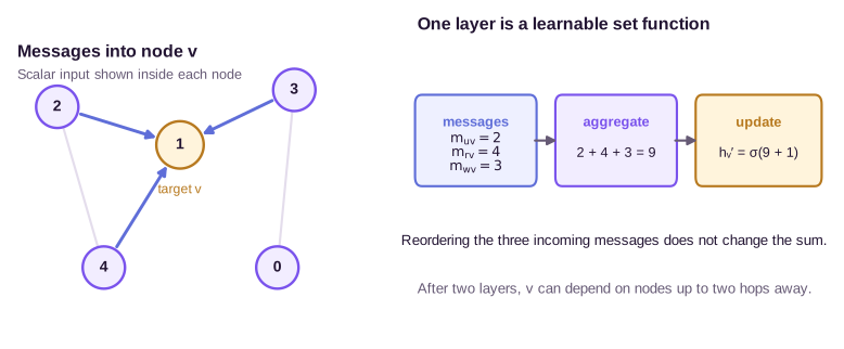
Consider the toy graph below. Each node starts with one scalar feature. The target node \(v\) has feature 1. Call its neighbors \(u\), \(r\), and \(w\), with features 2, 4, and 3. A fifth node \(q\) has feature 0 and connects only to \(w\). The undirected edges are

\[E=\{(u,v),(r,v),(w,v),(u,r),(w,q)\}.\]

The extra edges do not affect the first basic update at \(v\), but they determine degrees and allow \(q\) to reach \(v\) after two layers. We will keep this graph and these input features fixed when comparing architectures.

Let the first message function return the sender’s feature, let aggregation be a sum, and let the update add the old state before applying an activation:

\[m_{u\to v}=h_u, \qquad a_v=\sum_{u\in\mathcal{N}(v)}m_{u\to v}, \qquad h_v'=\sigma(a_v+h_v).\]

The aggregate is \(2+4+3=9\). With a ReLU activation, which is the identity on this positive input, the new state is \(h_v'=10\). Changing the order in which the three messages arrive does not change the result. These equations are a deliberately fixed, parameter-free update. The architecture comparisons below will state each additional learned parameter choice rather than quietly attributing it to the graph.

Receptive fields are powers of the propagation operator

The layer also defines a receptive field. To see the propagation explicitly, temporarily remove nonlinearities and learned channel mixing. Let \(\mathbf S\) be any matrix whose nonzero entry \(S_{vu}\) means that \(u\) sends to \(v\). A linear message-passing layer is

\[\mathbf H^{(1)}=\mathbf S\mathbf X,\]

and two layers give the exact identity

\[\mathbf H^{(2)}=\mathbf S^2\mathbf X, \qquad (\mathbf S^2)_{vq}=\sum_{w\in V}S_{vw}S_{wq}.\]

The coefficient from \(q\) to \(v\) is a sum over all length-two walks \(q\to w\to v\). On the five-node graph, there is exactly one such walk. Therefore \(q\) cannot affect \(v\) after one local layer, but it can after two. With nonlinearities, the update is no longer a matrix power, yet the support statement remains exact: after \(L\) layers, node \(v\) can depend only on nodes connected to it by a walk of length at most \(L\).

The receptive field describes possible dependence, not guaranteed information transfer. A path may receive zero learned weight, an activation may clip its signal, or several messages may cancel. Conversely, adding a virtual node or global attention changes the communication graph and can make distant nodes reachable in one or two layers.

Graph readout chooses whether size should matter

Graph-level prediction needs one more invariant operation. A readout such as

\[\mathbf{h}_G=\sum_{v\in V}\mathbf{h}_v^{(L)}\]

turns the final node states into one graph representation. An MLP can map \(\mathbf{h}_G\) to a molecular property, a graph class, or another global target. Node-level tasks skip this readout; edge-level tasks combine the states of the two incident nodes with their edge features.

Sum and mean readouts are both permutation invariant, but they encode different physical assumptions. Suppose the five final scalar node states happened to remain equal to their inputs. Their sum is 10 and their mean is 2. Now take the disjoint union of two identical copies. Sum readout becomes 20, while mean readout remains 2:

\[\operatorname{READOUT}_{\mathrm{sum}}(G\sqcup G) =2\operatorname{READOUT}_{\mathrm{sum}}(G), \qquad \operatorname{READOUT}_{\mathrm{mean}}(G\sqcup G) =\operatorname{READOUT}_{\mathrm{mean}}(G).\]

The sum is appropriate for an extensive target such as total energy or total mass, which scales with the number of independent components. The mean is appropriate for an intensive average such as mean node activity, provided the target truly should not scale with graph size. A learned MLP after mean pooling cannot recover the missing node count unless count is supplied separately. Invariance determines that node order must not matter; it does not determine whether graph size should matter.

Familiar architectures answer different aggregation failures

The common message-passing equation is more useful than a list of model names. It exposes which information each design preserves and which information it discards. GCN, GraphSAGE, GAT, and GIN can be read as answers to different weaknesses of a basic neighborhood average.

GCN: normalize repeated averaging

A GCN mixes each node with its neighbors using a normalized adjacency matrix (Kipf & Welling, 2017). Add self-loops to the graph,

\[\widetilde{\mathbf{A}}=\mathbf{A}+\mathbf{I},\]

and let \(\widetilde{\mathbf{D}}\) be its degree matrix. One GCN layer is

\[\mathbf{H}^{(\ell+1)} =\sigma\!\left( \widetilde{\mathbf{D}}^{-1/2} \widetilde{\mathbf{A}} \widetilde{\mathbf{D}}^{-1/2} \mathbf{H}^{(\ell)} \mathbf{W}^{(\ell)} \right).\]

The product by the normalized adjacency matrix is message aggregation; the product by \(\mathbf{W}^{(\ell)}\) is a learned feature transformation. An edge from \(u\) to \(v\) contributes with weight

\[\frac{1}{\sqrt{\widetilde d_u\widetilde d_v}},\]

so high-degree nodes neither send nor receive an unbounded sum merely because they have many neighbors. The matrix form also maps naturally to sparse matrix multiplication, giving a per-layer cost proportional to the number of edges rather than the number of possible node pairs.

The coefficient follows directly from two degree scalings. Define

\[\mathbf S =\widetilde{\mathbf D}^{-1/2} \widetilde{\mathbf A} \widetilde{\mathbf D}^{-1/2}.\]

Right multiplication by \(\widetilde{\mathbf D}^{-1/2}\) divides the feature sent by node \(u\) by \(\sqrt{\widetilde d_u}\). Left multiplication divides the aggregate received at \(v\) by \(\sqrt{\widetilde d_v}\). Expanding row \(v\) gives the identity

\[(\mathbf S\mathbf H)_v =\sum_{u:\,(u,v)\in\widetilde E} \frac{1}{\sqrt{\widetilde d_v\widetilde d_u}}\mathbf h_u.\]

The normalization is a fixed architectural choice. The feature matrix \(\mathbf W^{(\ell)}\) is learned. Keeping those roles separate matters: training can change how channels mix, but it cannot make one neighbor receive a different structural coefficient unless its degree differs or the architecture adds another weighting mechanism.

The matrix form also gives a compact symmetry check. Under relabeling, \(\widetilde{\mathbf A}'=\mathbf P\widetilde{\mathbf A}\mathbf P^{\mathsf T}\) and \(\widetilde{\mathbf D}'=\mathbf P\widetilde{\mathbf D}\mathbf P^{\mathsf T}\). Hence \(\mathbf S'=\mathbf P\mathbf S\mathbf P^{\mathsf T}\), and

\[\mathbf S'(\mathbf P\mathbf H)\mathbf W =\mathbf P\mathbf S\mathbf H\mathbf W.\]

Pointwise activation commutes with row permutation, so the entire GCN layer is equivariant.

The five-node GCN update

On our fixed graph, the self-loop degrees of \(v,u,r,w,q\) are \(4,3,3,3,2\). Set the one-dimensional learned weight to \(W=1\) and use the identity activation. These parameter choices isolate the propagation rule. The target update is

\[\begin{aligned} h_v^{\mathrm{GCN}} &=\frac{1}{4}(1) +\frac{1}{\sqrt{4\cdot3}}(2) +\frac{1}{\sqrt{4\cdot3}}(4) +\frac{1}{\sqrt{4\cdot3}}(3)\\ &=0.25+\frac{9}{\sqrt{12}} \approx2.848. \end{aligned}\]

The result is not the plain mean \((1+2+4+3)/4=2.5\). Symmetric normalization downweights the self-state more strongly than neighbor states because \(v\) has the larger degree. The same coefficients also make \(u\) and \(r\) structurally indistinguishable as senders to \(v\): their different numerical contributions come only from features 2 and 4.

Two layers make the fifth node reachable. In the linearized network, the coefficient multiplying the initial feature of \(q\) inside \(h_v^{(2)}\) is

\[(\mathbf S^2)_{vq} =S_{vw}S_{wq} =\frac{1}{\sqrt{4\cdot3}} \frac{1}{\sqrt{3\cdot2}} =\frac{1}{\sqrt{72}} \approx0.118.\]

Thus changing \(h_q^{(0)}\) from 0 to 5, while holding everything else fixed, increases the two-layer pre-activation at \(v\) by about \(0.589\). This is receptive-field propagation as a numerical coefficient rather than only a hop-count statement.

Normalization makes GCN stable and simple, but its weights are fixed once the graph is given. Two neighbors with the same degree receive the same structural coefficient even if one is relevant to the current prediction and the other is not.

GraphSAGE: make neighborhood computation inductive and bounded

GraphSAGE separates a node’s own state from an aggregated neighborhood state and can sample a fixed-size subset of neighbors (Hamilton et al., 2017). A mean-aggregating version has the form

\[\mathbf{a}_v^{(\ell)} =\frac{1}{\lvert S_v\rvert} \sum_{u\in S_v}\mathbf{h}_u^{(\ell-1)},\] \[\mathbf{h}_v^{(\ell)} =\sigma\!\left( \mathbf{W}^{(\ell)} \left[ \mathbf{h}_v^{(\ell-1)}\,\Vert\,\mathbf{a}_v^{(\ell)} \right] \right),\]

where \(S_v\subseteq\mathcal{N}(v)\) is a sampled neighborhood and \(\Vert\) denotes concatenation. The model learns a function of features rather than one embedding parameter per training node. It can therefore embed an unseen node, or a node in a new graph, provided the feature semantics remain compatible.

Sampling changes computation as well as statistics. A node with one million neighbors no longer forces every layer to inspect all one million. The sampled aggregate is noisy, and rare but decisive neighbors can be missed. GraphSAGE makes that trade explicit instead of hiding it behind a dense operation.

On the controlled graph, use the full neighborhood \(S_v=\{u,r,w\}\). The mean is

\[a_v^{\mathrm{SAGE}}=\frac{2+4+3}{3}=3.\]

Choose a one-output linear map \(\mathbf W=[1,1]\) and again use the identity activation. Concatenating the center and neighborhood values gives

\[h_v^{\mathrm{SAGE}} =\begin{bmatrix}1&1\end{bmatrix} \begin{bmatrix}1\\3\end{bmatrix} =4.\]

The value 4 is not an intrinsic output of GraphSAGE. It follows from the stated learned weights. What the architecture fixes is that the neighborhood contributes through its mean and that the center occupies a separate channel before learned mixing. Duplicating every neighbor would leave the mean at 3, whereas the original sum update would double the aggregate from 9 to 18.

Sampling one neighbor makes the tradeoff visible. A uniform one-sample estimate of the mean is 2, 4, or 3 with equal probability. It is unbiased because its expectation is 3, but its variance is

\[\frac{(2-3)^2+(4-3)^2+(3-3)^2}{3} =\frac{2}{3}.\]

Sampling bounds computation but replaces the exact neighborhood statistic with a random estimate. Sampling without a correction is not necessarily unbiased for attention, maximum, or a nonlinear function of the sampled set.

GAT: learn which neighbors matter

A GAT replaces fixed normalization with content-dependent weights (Veličković et al., 2018). It scores an ordered edge using the transformed sender and receiver states:

\[e_{uv} =\operatorname{LeakyReLU}\!\left( \mathbf{a}^{\mathsf T} \left[ \mathbf{W}\mathbf{h}_u\,\Vert\, \mathbf{W}\mathbf{h}_v \right] \right).\]

The scores are normalized across the neighbors of \(v\),

\[\alpha_{uv} =\frac{\exp(e_{uv})} {\sum_{w\in\mathcal{N}(v)}\exp(e_{wv})},\]

and the update is a weighted sum:

\[\mathbf{h}_v' =\sigma\!\left( \sum_{u\in\mathcal{N}(v)} \alpha_{uv}\mathbf{W}\mathbf{h}_u \right).\]

Softmax is itself invariant to the order in which the neighbor scores are listed, so attention does not break graph symmetry. It lets the model give different weights to different neighbors, but a high attention weight is not automatically a causal explanation. The weight is one internal routing coefficient, entangled with the value vectors and subsequent nonlinear layers.

The five-node graph gives a concrete attention calculation. Use one scalar channel, set \(W=1\), and choose the attention vector so that the positive-logit score is simply the sender feature: \(e_{uv}=h_u\). This is one possible learned parameter setting, not a GAT identity. For the three messages into \(v\), the logits are 2, 4, and 3. Their softmax weights are

\[(\alpha_{uv},\alpha_{rv},\alpha_{wv}) =\frac{(e^2,e^4,e^3)}{e^2+e^4+e^3} \approx(0.090,0.665,0.245).\]

With identity activation, the target receives

\[h_v^{\mathrm{GAT}} =0.090(2)+0.665(4)+0.245(3) \approx3.575.\]

GCN gave the feature-4 neighbor the same edge coefficient as the feature-2 neighbor because their degrees match. GAT assigns it more weight because the chosen learned score depends on content. The softmax also makes the update a weighted average: duplicating all three neighbors with identical copies leaves the output unchanged, because the numerator and denominator both double.

GIN: preserve multiplicity before asking an MLP to reason

Mean aggregation cannot distinguish multisets that have the same average. The neighbor features \(\{1,3\}\) and \(\{1,1,3,3\}\) both have mean 2, even though the second neighborhood contains twice as many nodes. Maximum aggregation loses even more multiplicity information.

GIN uses a sum followed by an MLP to retain as much multiset information as possible (Xu et al., 2019):

\[\mathbf{h}_v^{(\ell)} =\operatorname{MLP}^{(\ell)}\!\left( (1+\epsilon^{(\ell)})\mathbf{h}_v^{(\ell-1)} +\sum_{u\in\mathcal{N}(v)}\mathbf{h}_u^{(\ell-1)} \right).\]

The scalar \(\epsilon^{(\ell)}\) controls the distinction between the center node and its neighbors. Under suitable assumptions, the sum-plus-MLP construction can be injective on bounded multisets. This gives GIN the distinguishing power of the one-dimensional Weisfeiler–Lehman (1-WL) graph isomorphism test within the standard message-passing class.

For the shared graph, set \(\epsilon=0\) and let the MLP be the identity on our scalar input. Then

\[h_v^{\mathrm{GIN}}=1+(2+4+3)=10.\]

The numerical equality with the first basic sum update is deliberate: under these parameter choices, the two functions are identical at \(v\). GIN’s architectural claim concerns what the subsequent MLP can learn from a sum that retains multiplicity. It does not prescribe that the trained output must be 10.

Multiplicity and degree separate the aggregators

The controlled calculation can now be summarized without changing input data:

update at \(v\)	fixed aggregation result	stated learned choice	output
plain sum	\(2+4+3=9\)	add center, identity activation	\(10\)
GCN	degree-normalized self and neighbors	\(W=1\)	\(2.848\)
GraphSAGE	neighbor mean \(=3\)	\(W=[1,1]\)	\(4\)
GAT	learned weighted mean	sender-feature logits, \(W=1\)	\(3.575\)
GIN	neighbor sum \(=9\)	\(\epsilon=0\), identity MLP	\(10\)

The table compares mechanisms, not trained model quality. Its numbers depend on declared parameter choices, while the information retained by each aggregation rule is architectural.

Consider two neighbor multisets \(\{1,3\}\) and \(\{1,1,3,3\}\). Sum maps them to 4 and 8, so it preserves this change in multiplicity. Mean maps both to 2. Maximum maps both to 3. Softmax attention also maps them to the same weighted average whenever each distinct value is duplicated by the same factor: duplicating logits multiplies both the numerator and denominator by two.

These collisions have different meanings. Mean suppresses degree and estimates a local average. That can improve transfer across graph sizes when degree itself is nuisance variation. Sum retains degree-like count information but can grow with neighborhood size, so downstream layers must operate across a wider scale. Maximum detects whether a strong feature is present but forgets how often it occurs. Attention learns relative importance, yet its normalization still discards uniform replication of the entire multiset unless degree enters through another feature or channel.

No aggregator is universally best. The target decides whether multiplicity is signal. Counting functional groups in a molecule favors sum-like information. Estimating the average opinion among sampled contacts may favor a mean. Detecting the presence of one hazardous motif can favor a maximum. The symmetry condition requires order invariance; it does not choose which multiset distinctions to preserve.

That result is a ceiling, not a claim that GIN uniquely solves graph learning. GCN’s smoothing can be the right bias for homophilous node classification. Neighbor sampling can matter more than perfect multiset discrimination on a large graph. Attention can help when edge relevance varies with node state. Architecture choice is a choice about the information and computation that a task needs.

Global attention removes locality, not the symmetry constraint

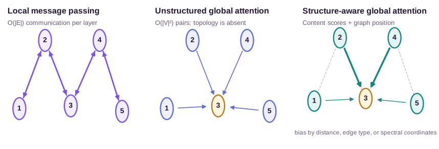
Local message passing is economical because it follows the edges. Its weakness is equally direct: a node needs many layers to receive information from a distant node. A Transformer allows every node to attend to every other node in one layer.

For query node \(v\) and source node \(u\), standard scaled dot-product attention uses

\[s_{uv} =\frac{(\mathbf{W}_Q\mathbf{h}_v)^{\mathsf T} (\mathbf{W}_K\mathbf{h}_u)}{\sqrt{d_k}}, \qquad \alpha_{uv}=\operatorname{softmax}_{u}(s_{uv}),\]

then forms

\[\mathbf{h}_v' =\sum_{u\in V}\alpha_{uv}\mathbf{W}_V\mathbf{h}_u.\]

With shared parameters and no sequence-specific positions, this operation is permutation equivariant. It also has no access to \(\mathbf{A}\). If every node begins with the same feature, an unstructured Transformer sees an unordered set of identical vectors whether the underlying graph is a chain, a ring, or two disconnected components.

Graph Transformers must therefore add positional or structural information. One strategy gives each node coordinates derived from eigenvectors of the graph Laplacian

\[\mathbf{L}=\mathbf{D}-\mathbf{A}, \qquad \mathbf{L}\mathbf{q}_k=\lambda_k\mathbf{q}_k.\]

The values \(q_k(v)\) from several low-frequency eigenvectors form a positional encoding for node \(v\). These coordinates describe slowly varying directions over the graph, much as sinusoidal coordinates describe low-frequency variation along a sequence. Unlike sequence positions, Laplacian eigenvectors are not uniquely oriented: each eigenvector can flip sign, and repeated eigenvalues allow rotations within an eigenspace. A model must account for those ambiguities rather than treating the coordinates as absolute labels.

A second strategy changes the pairwise attention score:

\[s_{uv} =\frac{(\mathbf{W}_Q\mathbf{h}_v)^{\mathsf T} (\mathbf{W}_K\mathbf{h}_u)}{\sqrt{d_k}} +b_{uv}.\]

The bias \(b_{uv}\) can encode shortest-path distance, edge types along a path, or whether two nodes are adjacent. Graphormer combines several such structural encodings with global attention (Ying et al., 2021). The attention remains global, but graph relations shape which global pairs are easy to use.

A shortest-path bias on the five-node graph

The controlled graph exposes what the bias contributes. Set every node feature to the same scalar for this calculation. Shared query and key maps then produce the same content score for every pair, so unstructured attention from \(v\) is uniform:

\[\alpha_{uv}=\frac{1}{5} \qquad\text{for every }u\in V.\]

The chain, the triangle-like connection among \(u,r,v\), and the two-hop node \(q\) are invisible. This is an exact consequence of identical inputs, not a failure that training can resolve: equal queries and keys produce equal dot products for any shared parameters.

Now define the learned structural form \(b_{uv}=-\gamma d_G(u,v)\), where \(d_G\) is shortest-path distance. Choose \(\gamma=\log 2\) only to make the arithmetic readable. The unnormalized weight becomes

\[\exp(b_{uv})=2^{-d_G(u,v)}.\]

Distances from \(v\) to \((v,u,r,w,q)\) are \((0,1,1,1,2)\). The unnormalized weights are therefore \((1,\frac12,\frac12,\frac12,\frac14)\) and sum to \(\frac{11}{4}\). After normalization,

\[(\alpha_{vv},\alpha_{uv},\alpha_{rv},\alpha_{wv},\alpha_{qv}) =\left(\frac4{11},\frac2{11},\frac2{11},\frac2{11},\frac1{11}\right).\]

Node \(q\) can now influence \(v\) in one layer, unlike local message passing, but the graph bias assigns it half the weight of a direct neighbor. The choice \(-\gamma d_G\) is a learned modeling family, not a graph identity. Another task may need a non-monotone distance table, edge-type bias, or no distance decay. Structural bias restores a relation that complete attention otherwise discards; it does not prove that shortest-path distance is the right relation for the target.

Laplacian positional encodings make a complementary choice. They attach node-wise coordinates rather than pairwise distances. The sign and repeated-eigenspace ambiguities described above mean that those coordinates cannot be treated like fixed sequence indices. Pairwise shortest-path bias avoids eigenvector sign choices, but it compresses all paths of the same length unless augmented with edge or path features.

The three communication patterns are contrasted below. Global attention is not simply a more expensive GAT. GAT normalizes over a graph-defined neighborhood; global attention defines a complete communication graph, then relies on structural features or biases to recover the distinctions that the complete graph erased.

In practice, local and global computation are complementary. GraphGPS combines a local message-passing block, a global attention block, and positional or structural encodings (Rampášek et al., 2022). The local block preserves the strong prior that observed edges matter. The global block creates short routes for long-range interaction. The encoding tells both blocks where nodes sit in the graph.

Sparse and dense communication have different scaling laws

Let node states have width \(d\) and let the graph have \(n\) nodes and \(m\) directed message edges. A local layer computes messages on existing edges, costing roughly \(O(md)\) once feature projections are available. Dense feature projections cost \(O(nd^2)\). The layer therefore costs

\[O(nd^2+md)\]

and stores edge-level activations of order \(O(md)\). Constants depend on the message function, but sparsity enters through \(m\).

Full self-attention forms all query-key scores. Projection still costs \(O(nd^2)\), while pairwise scores and weighted values cost \(O(n^2d)\) and attention memory is \(O(n^2)\) per head before implementation-specific savings. The dense layer costs

\[O(nd^2+n^2d).\]

For an undirected graph with average degree \(\bar k\), directed message count is approximately \(m=n\bar k\). With \(n=10{,}000\) and \(\bar k=20\), local propagation evaluates about \(200{,}000\) directed relations. Global attention evaluates \(100{,}000{,}000\) ordered pairs, a factor of 500 more before accounting for heads. One global layer shortens every communication path, but its pair count can dominate memory long before arithmetic becomes the only concern.

Depth changes the comparison. An \(L\)-layer local network costs about \(L\) times the sparse-layer cost and reaches at most \(L\) hops. If sampled GraphSAGE uses fanout \(s\) at every layer for one seed node, the naive computation tree contains up to \(s^L\) sampled occurrences, although implementations reuse repeated nodes. A hybrid model spends sparse computation on local chemistry or topology and reserves dense or approximate global computation for long-range interactions. Sparse global tokens, clustered attention, and low-rank kernels reduce cost by imposing another choice about which communication paths to preserve.

What the shared abstraction buys

Message passing gives graph learning four useful properties at once.

First, parameter sharing makes the model independent of graph size. The same message and update functions can process a molecule with 10 atoms or 100 atoms. Second, invariant aggregation removes dependence on arbitrary node order. Third, following observed edges gives sparse complexity, commonly proportional to \(\lvert E\rvert\) per layer. Fourth, the learned computation is inductive: it can be applied to a new graph without assigning a new parameter vector to every new node.

The abstraction also separates representation from prediction. The same stack of message-passing layers can support node classification, edge prediction, or graph regression by changing the readout. Edge attributes fit naturally because the message function receives \(\mathbf{e}_{uv}\). Directed or typed relations fit by giving different edge directions or relation types different transformations.

Architecture fixes a function family, not a fitted function

The controlled examples make three levels of a graph model easier to separate.

An identity follows from the mathematical object. Relabeling gives \(\mathbf A'=\mathbf P\mathbf A\mathbf P^{\mathsf T}\). Two linear propagation steps give \(\mathbf S^2\mathbf X\). Neither statement is learned.

An architectural assumption restricts the function family before training. GCN selects symmetric degree normalization. Mean GraphSAGE discards uniform replication of a neighborhood. GAT normalizes learned logits to a weighted average. GIN exposes a sum to an MLP. Global attention permits every ordered node pair to communicate. Data cannot make a mean aggregator recover multiplicity that it has already removed, although another channel can explicitly supply degree.

A learned choice is a parameter value inside that family. Our examples used \(W=1\) for GCN, \([1,1]\) for GraphSAGE, sender features as GAT logits, and an identity GIN MLP. Training will almost never return exactly those values. They were controlled interventions that exposed what each architecture does to the same input.

This separation prevents two common mistakes. The first is to call a numerical output an inherent property of a model name; the five-node GAT produced 3.575 only under our selected logits. The second is to expect optimization to undo an information bottleneck imposed before the learned function. Once mean pooling maps \(\{1,3\}\) and \(\{1,1,3,3\}\) to the same vector, every deterministic downstream MLP receives the same input and must return the same output.

These benefits explain why message passing became the default language of graph neural networks. They do not make it a universal solution.

What message passing misses

The most precise limitation is structural indistinguishability. If two nodes begin with the same state and receive the same multiset of neighbor states at every layer, a standard message-passing network keeps their states equal. At graph level, there are non-isomorphic graphs that 1-WL cannot distinguish, so GIN and other standard message-passing networks cannot distinguish them from uniform initial features either. Higher-order GNNs, subgraph features, and positional encodings add information beyond the node-centered multiset. The dedicated post How Expressive Are Graph Neural Networks? develops this boundary with explicit indistinguishable graph pairs.

Depth does not cheaply fix the problem. Repeated neighborhood averaging can make node representations converge toward similar values, a phenomenon called over-smoothing (Oono & Suzuki, 2020). Residual connections and identity-preserving updates help optimization, but they do not change the fact that many smoothing steps can erase local distinctions.

Long-range dependency creates a different failure. The number of nodes in an \(L\)-hop neighborhood can grow exponentially with \(L\), while the receiving node has a fixed-width vector. Information from many distant nodes must be compressed through narrow graph cuts into that vector. This over-squashing can prevent the model from representing a dependency even before over-smoothing makes all nodes look alike. Rewiring, hierarchical representations, global states, and attention create shorter or wider communication paths; none is free of computational or modeling tradeoffs (Topping et al., 2022). Deep Graph Network Failure Modes treats over-smoothing, over-squashing, bottlenecks, and their remedies as the main subject.

The observed graph may also be the wrong computational graph. A molecular bond graph records covalent bonds, but electrostatic interactions need not follow bond distance. A social edge can represent disagreement rather than similarity. A protein contact map may omit geometric direction and distance. A message-passing network faithfully follows the edges it receives; it cannot infer missing relation semantics merely from the promise that the input is a graph.

Graph Transformers address some long-range limits, but they trade sparse computation for pairwise interaction. Full attention costs quadratically in the number of nodes. Approximate attention, sparsification, and hybrid local–global designs recover scalability by deciding which global interactions to retain. That decision becomes another graph prior.

The useful question is what information should move

Graph neural networks are often introduced as convolutions generalized from grids. The stronger view starts from symmetry. Node indices are arbitrary, so a graph layer must commute with node relabeling. Shared edge functions and invariant neighborhood aggregation satisfy that constraint, giving the message-passing template.

GCN normalizes a fixed local average. GraphSAGE makes neighborhood computation inductive and sampleable. GAT learns relative weights within the observed neighborhood. GIN protects multiplicity so an MLP can distinguish richer multisets. A graph Transformer opens communication beyond observed edges, then must restore topology through positional features or pairwise structural biases.

The shared abstraction turns architecture names into design questions. Which relations should permit communication? What must a message contain? Which information may the aggregator discard? How far must information travel, and through how narrow a channel? Those questions survive the next model name because they come from the graph itself.

References

• Gilmer, J., Schoenholz, S. S., Riley, P. F., Vinyals, O., & Dahl, G. E. (2017). Neural Message Passing for Quantum Chemistry. Proceedings of Machine Learning Research. ↩
• Kipf, T. N., & Welling, M. (2017). Semi-Supervised Classification with Graph Convolutional Networks. ICLR. ↩
• Hamilton, W. L., Ying, R., & Leskovec, J. (2017). Inductive Representation Learning on Large Graphs. NeurIPS. ↩
• Veličković, P., Cucurull, G., Casanova, A., Romero, A., Liò, P., & Bengio, Y. (2018). Graph Attention Networks. ICLR. ↩
• Xu, K., Hu, W., Leskovec, J., & Jegelka, S. (2019). How Powerful Are Graph Neural Networks? ICLR. ↩
• Ying, C., Cai, T., Luo, S., Zheng, S., Ke, G., He, D., Shen, Y., & Liu, T.-Y. (2021). Do Transformers Really Perform Badly for Graph Representation? NeurIPS. ↩
• Rampášek, L., Galkin, M., Dwivedi, V. P., Luu, A. T., Wolf, G., & Beaini, D. (2022). Recipe for a General, Powerful, Scalable Graph Transformer. NeurIPS. ↩
• Oono, K., & Suzuki, T. (2020). Graph Neural Networks Exponentially Lose Expressive Power for Node Classification. ICLR. ↩
• Topping, J., Di Giovanni, F., Chamberlain, B. P., Dong, X., & Bronstein, M. M. (2022). Understanding Over-Squashing and Bottlenecks on Graphs via Curvature. ICLR. ↩