Two Routes to Graph Convolution

Adapted from my 2025 Geometric Deep Learning lectures. Rather than asking how to implement message passing, this article derives graph convolution twice—through spectral filtering and permutation equivariance—and shows exactly where the two routes meet.

A convolution is not defined by sliding a small window. The sliding-window formula is a consequence of a stronger statement: convolution is a linear map that commutes with translation. Shift the input and then convolve, or convolve and then shift; either route gives the same output.

This definition gives us two routes from ordinary convolution to graph convolution. The first replaces the frequencies of a regular grid with the eigenvectors of a graph Laplacian. A convolution then becomes a spectral filter, and locality appears when we approximate that filter by a polynomial. The second route starts from symmetry alone. It asks which linear maps commute with every permutation of the nodes, turning equivariance into a fixed-point problem.

The two routes meet near familiar graph neural network layers, but they are not interchangeable. Spectral filtering describes variation relative to one graph. Permutation equivariance describes how a model should behave when any graph is relabeled. Understanding both explains why the graph convolutional network (GCN) update is natural, why it transfers across graphs despite its spectral origin, and why message passing needs the adjacency matrix as an input rather than as a hidden coordinate system.

Convolution is a commutation relation

Consider a one-dimensional periodic signal \(\mathbf{x}\in\mathbb{R}^{N}\). Let \(\mathbf{S}\) be the cyclic shift matrix, so \((\mathbf{S}\mathbf{x})_i=x_{i-1}\) with indices interpreted modulo \(N\). A linear map \(\mathbf{C}\) is shift equivariant when

\[\mathbf{C}\mathbf{S}\mathbf{x} =\mathbf{S}\mathbf{C}\mathbf{x} \qquad\text{for every }\mathbf{x}.\]

Because this equality holds for every input, it is equivalent to the matrix relation

\[\mathbf{C}\mathbf{S}=\mathbf{S}\mathbf{C}.\]

In other words, \(\mathbf{C}\) lies in the commutant of the shift: the set of linear maps that commute with \(\mathbf{S}\). For a cyclic signal, these maps are exactly the circulant matrices. Each row is a shifted copy of the previous row, so the same weights are reused at every location. Multiplication by a circulant matrix is circular convolution.

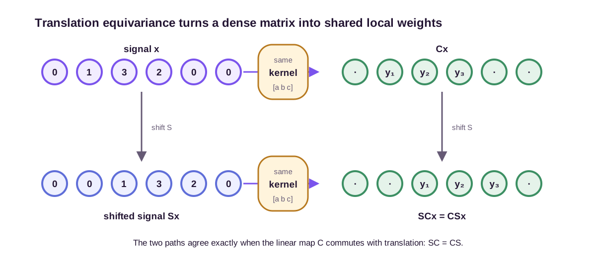
This perspective separates the mathematical property from its implementation. Local support is common because small filters are efficient and encode locality, but shift equivariance itself only requires a circulant matrix. A circulant kernel can span the entire periodic signal. Conversely, a locally connected layer whose weights vary with position is local but not shift equivariant.

The Fourier transform makes the commutant easy to describe. The cyclic shift is diagonalized by the discrete Fourier basis. Every circulant matrix has the same eigenvectors, so it acts by multiplying each Fourier coefficient by a scalar. Convolution in the signal domain and pointwise multiplication in the frequency domain are two descriptions of the same operator.

The constraint is visible on four sites. With the convention \((\mathbf S\mathbf x)_i=x_{i-1}\) modulo four, choose the first column of \(\mathbf C\) as \((a,b,c,d)^{\mathsf T}\). Commutation forces every later column to be its cyclic shift:

\[\mathbf C= \begin{pmatrix} a&d&c&b\\ b&a&d&c\\ c&b&a&d\\ d&c&b&a \end{pmatrix}.\]

A generic \(4\times4\) matrix has 16 parameters; the shift commutant has four. For an impulse \(\mathbf e_1\), the output is the kernel \((a,b,c,d)^{\mathsf T}\) itself. Shifting the impulse selects the next column, which is exactly the shifted output. This finite calculation is the weight-sharing theorem in matrix form, without an appeal to an infinite grid.

This suggests a graph analogue. We need an operator that measures frequency on an irregular domain, and we need its eigenvectors to replace the sines and cosines.

The graph Laplacian defines frequency

Let \(G=(V,E)\) be an undirected weighted graph with \(N\) nodes. Its symmetric adjacency matrix is \(\mathbf{A}\in\mathbb{R}^{N\times N}\), where \(A_{ij}\geq 0\) is the weight of edge \((i,j)\). Let \(\mathbf{D}\) be the diagonal degree matrix, with \(D_{ii}=\sum_j A_{ij}\). The combinatorial graph Laplacian is

\[\mathbf{L}=\mathbf{D}-\mathbf{A}.\]

A graph signal assigns one scalar to each node, so we write it as \(\mathbf{f}\in\mathbb{R}^{N}\). Applying the Laplacian compares each value with its neighbors:

\[(\mathbf{L}\mathbf{f})_i =\sum_{j=1}^{N}A_{ij}(f_i-f_j).\]

The quadratic form of the Laplacian measures total variation across edges:

\[\mathbf{f}^{\mathsf T}\mathbf{L}\mathbf{f} =\frac{1}{2}\sum_{i,j=1}^{N}A_{ij}(f_i-f_j)^2.\]

Signals that change little across strongly weighted edges have small quadratic form. Signals that alternate sharply between adjacent nodes have large quadratic form. The Laplacian therefore supplies the notion of smoothness that a graph lacks as a coordinate-free object.

Because \(\mathbf{L}\) is real and symmetric, it has an orthonormal eigendecomposition

\[\mathbf{L}=\mathbf{U}\boldsymbol{\Lambda}\mathbf{U}^{\mathsf T},\]

where \(\boldsymbol{\Lambda}=\operatorname{diag}(\lambda_0,\ldots,\lambda_{N-1})\) contains nonnegative eigenvalues in ascending order, and the columns \(\mathbf{u}_0,\ldots,\mathbf{u}_{N-1}\) of \(\mathbf{U}\) are the corresponding eigenvectors. If the graph is connected, \(\lambda_0=0\) and \(\mathbf{u}_0\) is constant. Larger eigenvalues correspond to eigenvectors with greater edge-wise variation because

\[\mathbf{u}_{\ell}^{\mathsf T}\mathbf{L}\mathbf{u}_{\ell} =\lambda_{\ell}.\]

The eigenvectors of \(\mathbf{L}\) are the graph Fourier basis (Shuman et al., 2013). The graph Fourier transform and its inverse are

\[\widehat{\mathbf{f}}=\mathbf{U}^{\mathsf T}\mathbf{f}, \qquad \mathbf{f}=\mathbf{U}\widehat{\mathbf{f}}.\]

The coefficient \(\widehat{f}_{\ell}=\mathbf{u}_{\ell}^{\mathsf T}\mathbf{f}\) measures how much of the \(\ell\)-th Laplacian mode appears in the signal. The analogy with ordinary Fourier analysis is exact at the level we need: the Laplacian provides modes ordered by variation, and the transform expresses a signal in those modes.

One impulse on the three-node path

Use the path \(1\!-!2\!-!3\) throughout the spectral derivation. Its combinatorial Laplacian is

\[\mathbf L= \begin{pmatrix} 1&-1&0\\ -1&2&-1\\ 0&-1&1 \end{pmatrix}.\]

An orthonormal eigensystem is

\[\begin{array}{c|c} \lambda&\mathbf u^{\mathsf T}\\ \hline 0&(1,1,1)/\sqrt3\\ 1&(1,0,-1)/\sqrt2\\ 3&(1,-2,1)/\sqrt6 \end{array}.\]

Direct multiplication verifies \(\mathbf L\mathbf u_{\ell}=\lambda_{\ell}\mathbf u_{\ell}\). Now place a unit impulse at the first endpoint, \(\mathbf f=\mathbf e_1=(1,0,0)^{\mathsf T}\). Its graph Fourier coefficients are the first entries of the eigenvectors:

\[\widehat{\mathbf f} =\left(\frac1{\sqrt3},\frac1{\sqrt2},\frac1{\sqrt6}\right)^{\mathsf T}.\]

The impulse contains every mode. Its largest coefficient is on the middle-frequency antisymmetric mode, while the constant and highest-frequency modes are also present. Every filter below will act on this same signal, so differences in output come from the operator rather than from a changed example.

Spectral filtering becomes graph convolution

A spectral filter multiplies each Fourier coefficient by a response \(h(\lambda_{\ell})\). In matrix form,

\[\widehat{g}_{\ell}=h(\lambda_{\ell})\widehat{f}_{\ell},\]

and therefore

\[\mathbf{g} =\mathbf{U}h(\boldsymbol{\Lambda})\mathbf{U}^{\mathsf T}\mathbf{f} =h(\mathbf{L})\mathbf{f}.\]

Here \(h(\boldsymbol{\Lambda})\) is diagonal, with entry \(h(\lambda_{\ell})\) at mode \(\ell\). A low-pass filter assigns smaller multipliers to larger eigenvalues, suppressing signals that vary rapidly across edges. A high-pass filter does the reverse.

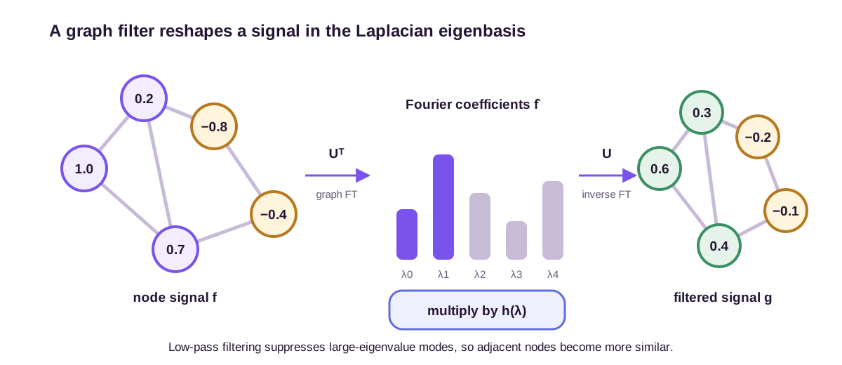
This definition is often called spectral graph convolution. It is a reasonable analogue of ordinary convolution because the operator is diagonal in the graph Fourier basis. It also commutes with the Laplacian:

\[h(\mathbf{L})\mathbf{L}=\mathbf{L}h(\mathbf{L}).\]

The statement needs one qualification. If all eigenvalues are distinct, every matrix that commutes with \(\mathbf{L}\) is diagonal in its eigenbasis and can be written as a function on its finite spectrum. With repeated eigenvalues, the full commutant can also mix vectors inside a repeated eigenspace. A scalar response \(h(\lambda)\) selects the basis-independent subset that treats an entire eigenspace uniformly.

That distinction resolves a common problem with Laplacian eigenvectors. An individual eigenvector has an arbitrary sign: both \(\mathbf{u}_{\ell}\) and \(-\mathbf{u}_{\ell}\) are valid. A repeated eigenspace has a larger ambiguity because any orthogonal rotation within it is valid. The operator \(h(\mathbf{L})\) is unaffected by either choice. Using individual eigenvectors as positional features requires explicit handling of sign and basis ambiguity; using a scalar spectral filter does not.

On the three-node path, choose the rational low-pass response

\[h(\lambda)=\frac{1}{1+\lambda}.\]

The multipliers at eigenvalues \((0,1,3)\) are \((1,1/2,1/4)\). Applying them to the impulse coefficients and reconstructing gives

\[\begin{aligned} h(\mathbf L)\mathbf e_1 &=\frac13(1,1,1)^{\mathsf T} +\frac14(1,0,-1)^{\mathsf T} +\frac1{24}(1,-2,1)^{\mathsf T}\\ &=\left(\frac58,\frac14,\frac18\right)^{\mathsf T}. \end{aligned}\]

Equivalently, this output solves \((\mathbf I+\mathbf L)\mathbf g=\mathbf e_1\). The positive mass reaches node 3 even though it is two hops from the impulse because the rational function corresponds to a dense inverse, not a finite-degree polynomial.

Repeated eigenvalues change the commutant

The four-cycle \(C_4\) has Laplacian eigenvalues \(0,2,2,4\). One basis for the repeated \(\lambda=2\) eigenspace is

\[\mathbf v_1=(1,0,-1,0)^{\mathsf T}/\sqrt2, \qquad \mathbf v_2=(0,1,0,-1)^{\mathsf T}/\sqrt2.\]

For any \(2\times2\) orthogonal matrix \(Q\), the columns of \((\mathbf v_1,\mathbf v_2)Q\) are an equally valid eigenbasis. A matrix commuting with \(\mathbf L\) may apply an arbitrary linear \(2\times2\) map inside this repeated eigenspace; if the commuting matrix is also symmetric, that block must be symmetric but need not be scalar. By contrast, a scalar filter \(h(\mathbf L)\) applies exactly \(h(2)\mathbf I_2\) there. It cannot distinguish a rotated choice of \(\mathbf v_1\) and \(\mathbf v_2\).

For example, define an operator that is zero on the \(\lambda=0\) and \(\lambda=4\) modes and acts on \((\mathbf v_1,\mathbf v_2)\) by

\[\mathbf M= \begin{pmatrix}1&1/2\\1/2&2\end{pmatrix}.\]

This symmetric operator commutes with \(\mathbf L\) because \(\mathbf L\) is \(2\mathbf I\) on that subspace: \(\mathbf M(2\mathbf I)=(2\mathbf I)\mathbf M\). Yet it is not \(h(\mathbf L)\) for any scalar \(h\) because its two eigenvalues within the same Laplacian eigenspace differ. Rotating the basis conjugates the coordinate block to \(Q^{\mathsf T}\mathbf M Q\), while the underlying operator stays fixed. Writing a free diagonal multiplier in one arbitrary eigenbasis would not have that basis independence.

Thus “commutes with the Laplacian” is broader than “is a scalar function of the Laplacian” when eigenvalues repeat. The latter is basis-independent and transferable as a response rule; the former can encode a choice of coordinates inside a degenerate eigenspace.

Polynomial filters recover locality

Directly learning one free multiplier for each eigenvalue is a poor neural-network layer. It requires an eigendecomposition, uses \(N\) parameters tied to one graph size, and gives a dense operator in the node domain. A polynomial response avoids all three problems:

\[h_{\boldsymbol{\theta}}(\lambda) =\sum_{k=0}^{K}\theta_k\lambda^k.\]

Substituting \(\mathbf{L}=\mathbf{U}\boldsymbol{\Lambda}\mathbf{U}^{\mathsf T}\) gives

\[h_{\boldsymbol{\theta}}(\mathbf{L})\mathbf{f} =\sum_{k=0}^{K}\theta_k\mathbf{L}^{k}\mathbf{f}.\]

The eigenvectors disappear from the computation. The coefficients \(\theta_0,\ldots,\theta_K\) do not depend on the number of nodes, so the same filter can be applied to graphs of different sizes. The operator is also \(K\)-hop localized: multiplying by \(\mathbf{L}\) communicates along one edge, so \(\mathbf{L}^{k}\) cannot connect nodes more than \(k\) hops apart.

ChebNet uses Chebyshev polynomials rather than monomials because they provide a numerically stable approximation on a rescaled spectrum (Defferrard et al., 2016). If the spectrum is mapped to \([-1,1]\), the basis follows the recurrence

\[T_0(x)=1, \qquad T_1(x)=x, \qquad T_k(x)=2xT_{k-1}(x)-T_{k-2}(x).\]

A Chebyshev filter evaluates \(\sum_{k=0}^{K}\theta_kT_k(\widetilde{\mathbf{L}})\mathbf{f}\) recursively. It retains the spectral interpretation while requiring only sparse matrix-vector products.

This is the first bridge to message passing. A global frequency-domain definition becomes a local spatial computation after restricting the response to a polynomial. Locality is not inserted after the derivation; it follows from the algebra of powers of a sparse Laplacian.

Use the degree-one response \(p(\lambda)=1-\lambda/4\) on the same path impulse. Its spectral multipliers at \((0,1,3)\) are \((1,3/4,1/4)\), so it agrees with the rational filter at the endpoints of the spectrum but not at \(\lambda=1\). In the node domain,

\[p(\mathbf L)\mathbf e_1 =\left(\mathbf I-\frac14\mathbf L\right)\mathbf e_1 =\left(\frac34,\frac14,0\right)^{\mathsf T}.\]

Node 3 receives exactly zero because a degree-one polynomial cannot cross two edges. The rational output \((5/8,1/4,1/8)^{\mathsf T}\) is smoother and global; the polynomial output is localized and only approximates the desired response. Raising the degree expands both approximation capacity and receptive radius.

The GCN layer is a first-order spectral model

Kipf and Welling simplify the polynomial construction to obtain the graph convolutional network (Kipf and Welling, 2017). Start from the symmetric normalized Laplacian

\[\mathbf{L}_{\mathrm{sym}} =\mathbf{I}-\mathbf{D}^{-1/2}\mathbf{A}\mathbf{D}^{-1/2}.\]

A first-order spectral approximation can be reduced, after rescaling the spectrum and tying coefficients, to an operator proportional to

\[\mathbf{I}+\mathbf{D}^{-1/2}\mathbf{A}\mathbf{D}^{-1/2}.\]

Repeatedly applying this operator can create unstable scales. The practical GCN uses a renormalization trick: add one self-loop to every node and normalize the resulting adjacency. Define

\[\widetilde{\mathbf{A}}=\mathbf{A}+\mathbf{I}, \qquad \widetilde{D}_{ii}=\sum_j\widetilde{A}_{ij},\]

and

\[\widehat{\mathbf{A}} =\widetilde{\mathbf{D}}^{-1/2} \widetilde{\mathbf{A}} \widetilde{\mathbf{D}}^{-1/2}.\]

For node features \(\mathbf{H}^{(k)}\in\mathbb{R}^{N\times d_k}\), one GCN layer is

\[\mathbf{H}^{(k+1)} =\sigma\!\left( \widehat{\mathbf{A}}\mathbf{H}^{(k)}\mathbf{W}^{(k)} \right),\]

where \(\mathbf{W}^{(k)}\in\mathbb{R}^{d_k\times d_{k+1}}\) mixes feature channels and \(\sigma\) is a pointwise nonlinearity. The left multiplication by \(\widehat{\mathbf{A}}\) mixes nodes; the right multiplication by \(\mathbf{W}^{(k)}\) mixes channels. Conflating these two operations makes the layer look more mysterious than it is.

For the three-node path and the same impulse \(\mathbf e_1\), adding self-loops gives degrees \((2,3,2)\). One propagation is

\[\widehat{\mathbf{A}}\mathbf{x} =\left( \frac{1}{2}, \frac{1}{\sqrt{6}}, 0 \right)^{\mathsf T}.\]

The first node retains half of its value, the second receives \(1/\sqrt6\approx0.408\), and node 3 remains zero. The degree-one combinatorial polynomial gave \((0.75,0.25,0)\); the two operators share one-hop support but not weights or normalization.

The approximation ledger

The path from ChebNet to this update contains several different logical moves. Write \(\mathbf S=\mathbf D^{-1/2}\mathbf A\mathbf D^{-1/2}\), so the exact identity \(\mathbf L_{\mathrm{sym}}=\mathbf I-\mathbf S\) holds.

1. Spectral rescaling is an exact definition once \(\lambda_{\max}\) is chosen. ChebNet sets

   \[\widetilde{\mathbf L}=\frac{2}{\lambda_{\max}}\mathbf L_{\mathrm{sym}}-\mathbf I,\]

   mapping the observed spectrum into \([-1,1]\) when \(\lambda_{\max}\) is the true largest eigenvalue.

2. First-order truncation is a restriction or approximation. Keeping \(K=1\) yields

   \[\theta_0T_0(\widetilde{\mathbf L})+\theta_1T_1(\widetilde{\mathbf L}) =\theta_0\mathbf I+\theta_1\widetilde{\mathbf L}.\]

   This is exact only for a target response already affine in the rescaled eigenvalue. For the rational response above, it is an approximation.

3. Setting \(\lambda_{\max}\approx2\) is a spectral approximation. The eigenvalues of a symmetric normalized Laplacian lie in \([0,2]\). With the substitution,

   \[\widetilde{\mathbf L}\approx\mathbf L_{\mathrm{sym}}-\mathbf I=-\mathbf S.\]

   For the bipartite three-node path, \(\lambda_{\max}=2\) exactly, so this step happens to be exact. It is not exact for every graph.

   The path check can be done without a bound. Its normalized adjacency and Laplacian are

   \[\mathbf S= \begin{pmatrix} 0&1/\sqrt2&0\\ 1/\sqrt2&0&1/\sqrt2\\ 0&1/\sqrt2&0 \end{pmatrix}, \qquad \mathbf L_{\mathrm{sym}}=\mathbf I-\mathbf S.\]

   The normalized-Laplacian eigenvalues are \(0,1,2\), with eigenvectors proportional to \((1,\sqrt2,1)\), \((1,0,-1)\), and \((1,-\sqrt2,1)\). Thus the substitution \(\lambda_{\max}=2\) is exact here even though the combinatorial Laplacian used earlier had largest eigenvalue 3. The symbol “Laplacian” does not identify a spectrum until its normalization is specified.

4. Coefficient tying is a design choice. Setting \(\theta_0=-\theta_1=\theta\) reduces two spectral parameters to one and gives \(\theta(\mathbf I+\mathbf S)\). Symmetry does not force this tying.

5. Renormalization is a replacement, not an algebraic simplification. The practical layer replaces \(\mathbf I+\mathbf S\) with

   \[\widehat{\mathbf A}=(\mathbf D+\mathbf I)^{-1/2}(\mathbf A+\mathbf I)(\mathbf D+\mathbf I)^{-1/2}.\]

   On the path impulse, \((\mathbf I+\mathbf S)\mathbf e_1=(1,1/\sqrt2,0)^{\mathsf T}\), whereas renormalization gives \((1/2,1/\sqrt6,0)^{\mathsf T}\). No single scalar converts both nonzero entries. Adding self-loops before recomputing degrees changes the operator.

The practical GCN is therefore motivated by a first-order spectral construction and then deliberately regularized. Calling the final matrix an exact Chebyshev identity hides the coefficient restriction and the renormalization design.

The normalization also encodes a choice of scale. Symmetric normalization weights an edge \((i,j)\) by \(1/\sqrt{\widetilde{d}_i\widetilde{d}_j}\), reducing the influence of hubs in either direction. It does not preserve a constant signal on an irregular graph. Random-walk normalization \(\widetilde{\mathbf{D}}^{-1}\widetilde{\mathbf{A}}\) does preserve constants but is generally not symmetric. These operators share a smoothing intuition, not identical dynamics.

The same impulse under five operators

The shared example now separates the constructions cleanly:

operator	output on \(\mathbf e_1\)	support	sum of entries
identity	\((1,0,0)\)	node 1	1
rational \((\mathbf I+\mathbf L)^{-1}\)	\((5/8,1/4,1/8)\)	all nodes	1
degree-one \(\mathbf I-\mathbf L/4\)	\((3/4,1/4,0)\)	one hop	1
tied pre-renormalization \(\mathbf I+\mathbf S\)	\((1,1/\sqrt2,0)\)	one hop	\(1+1/\sqrt2\)
self-loop GCN \(\widehat{\mathbf A}\)	\((1/2,1/\sqrt6,0)\)	one hop	\(1/2+1/\sqrt6\)

The first three use the combinatorial Laplacian and preserve total sum because their response at \(\lambda=0\) is one and the constant vector spans its nullspace. The symmetric-normalized operators preserve a degree-weighted mode instead, so ordinary mass need not remain one. Support alone cannot identify the derivation: the degree-one polynomial, pre-renormalized update, and GCN are all one-hop, yet their values differ.

Smoothing also needs a scale convention. For the unfiltered impulse, combinatorial Dirichlet energy is

\[\mathbf e_1^{\mathsf T}\mathbf L\mathbf e_1=1.\]

The rational output has edge differences \(3/8\) and \(1/8\), giving energy \(9/64+1/64=5/32\). The degree-one output has differences \(1/2\) and \(1/4\), giving \(1/4+1/16=5/16\). Both smooth the impulse, and the rational filter smooths more under this measure. Comparing the GCN energy directly would mix filtering with its changed normalization and overall scale; normalize the output or specify the operator before making that comparison.

A fixed spectrum does not explain graph relabeling

The spectral route begins with one Laplacian and defines frequency relative to it. This is natural for signals observed repeatedly on a fixed graph, such as measurements on one sensor network. It is less natural when each example has a different graph, as in molecular datasets.

Changing the graph changes its eigenvalues, eigenvectors, and often its number of nodes. A filter with one parameter per eigenvalue cannot be transferred directly. Polynomial filters repair much of this problem because their coefficients act through \(\mathbf{L}\) rather than through named eigenvectors. But the spectral story still does not state the basic data symmetry: relabeling a graph’s nodes should only relabel its node-wise output.

Polynomial filters do satisfy that symmetry when the graph and signal are relabeled together. Let \(\mathbf L'=\mathbf P\mathbf L\mathbf P^{\mathsf T}\) and \(\mathbf f'=\mathbf P\mathbf f\). Since \(\mathbf P^{\mathsf T}\mathbf P=\mathbf I\), induction gives

\[(\mathbf L')^k =(\mathbf P\mathbf L\mathbf P^{\mathsf T})^k =\mathbf P\mathbf L^k\mathbf P^{\mathsf T}.\]

Therefore, for \(p(\mathbf L)=\sum_{k=0}^K\theta_k\mathbf L^k\),

\[p(\mathbf L')\mathbf f' =\sum_k\theta_k\mathbf P\mathbf L^k\mathbf P^{\mathsf T}\mathbf P\mathbf f =\mathbf Pp(\mathbf L)\mathbf f.\]

This is an exact equivariance proof, not an appeal to eigenvector alignment. It requires simultaneous relabeling of the operator and signal and shared coefficients \(\theta_k\). Fixing \(\mathbf L\) while permuting only \(\mathbf f\) asks for a different symmetry: commutation with automorphisms of that fixed graph, not equivariance across labeled presentations.

That requirement leads to the second derivation.

Permutation equivariance is another commutant

First ignore the graph edges and consider a node signal \(\mathbf{x}\in\mathbb{R}^{N}\). A permutation matrix \(\mathbf{P}\) relabels its entries. A linear map \(\mathbf{C}\in\mathbb{R}^{N\times N}\) is permutation equivariant when

\[\mathbf{C}\mathbf{P}\mathbf{x} =\mathbf{P}\mathbf{C}\mathbf{x} \qquad\text{for every permutation }\mathbf{P} \text{ and every }\mathbf{x}.\]

Equivalently, \(\mathbf{C}\mathbf{P}=\mathbf{P}\mathbf{C}\) for every permutation matrix. This is again a commutant, now for the entire symmetric group rather than for one shift.

The constraint is severe. Permutations can move any diagonal entry of \(\mathbf{C}\) to any other diagonal position, so all diagonal entries must agree. They can also move any ordered pair of distinct indices to any other such pair, so all off-diagonal entries must agree. Therefore

\[\mathbf{C}=\alpha\mathbf{I}+\beta\mathbf{1}\mathbf{1}^{\mathsf T},\]

and the node-wise form is

\[y_i=\alpha x_i+\beta\sum_{j=1}^{N}x_j.\]

Every permutation-equivariant linear map on scalar node features is a combination of keeping each node’s own value and broadcasting a global sum. This is the linear core behind the Deep Sets characterization (Zaheer et al., 2017). It contains no neighborhood operation because we deliberately supplied no graph.

Apply this complete family to the path impulse, while still withholding the path adjacency:

\[\mathbf C\mathbf e_1 =\alpha\mathbf e_1+\beta\mathbf 1 =(\alpha+\beta,\beta,\beta)^{\mathsf T}.\]

Nodes 2 and 3 must receive the same value because a feature-only permutation can exchange them. The desired one-hop pattern \((3/4,1/4,0)\) and the GCN pattern \((1/2,1/\sqrt6,0)\) are impossible for every choice of \(\alpha,\beta\): making the third entry zero forces \(\beta=0\) and therefore also makes the second zero. This is an input-information limitation, not a weak choice of parameters.

Higher-order features turn equivariance into fixed points

An adjacency matrix has two node indices. Under relabeling it transforms as

\[\mathbf{X}\mapsto\mathbf{P}\mathbf{X}\mathbf{P}^{\mathsf T}.\]

Vectorization turns this action into multiplication by a Kronecker-product representation:

\[\operatorname{vec}(\mathbf{P}\mathbf{X}\mathbf{P}^{\mathsf T}) =(\mathbf{P}\otimes\mathbf{P})\operatorname{vec}(\mathbf{X}).\]

Let \(\mathcal{L}\) be a linear map from matrices to matrices, represented as a matrix acting on \(\operatorname{vec}(\mathbf{X})\). Equivariance requires

\[\mathcal{L}(\mathbf{P}\mathbf{X}\mathbf{P}^{\mathsf T}) =\mathbf{P}\mathcal{L}(\mathbf{X})\mathbf{P}^{\mathsf T}.\]

If \(\mathbf{R}_{\mathbf{P}}=\mathbf{P}\otimes\mathbf{P}\), the matrix representing \(\mathcal{L}\) must satisfy

\[\mathbf{R}_{\mathbf{P}}^{\mathsf T} \mathcal{L} \mathbf{R}_{\mathbf{P}} =\mathcal{L} \qquad\text{for every }\mathbf{P}.\]

After vectorizing once more, this becomes a fixed-point equation under a four-index permutation action. Write \(\mathcal{L}_{ij,k\ell}\) for the coefficient mapping input entry \(X_{k\ell}\) to output entry \((i,j)\). Equivariance forces coefficients with the same equality pattern among the four indices to agree. One basis pattern has \(i=j=k=\ell\). Another has \(i=j\) and \(k=\ell\) but \(i\neq k\). For a map between order-\(p\) and order-\(q\) tensors, the stable dimension is the Bell number \(B_{p+q}\) when \(N\ge p+q\), because every partition of the index positions can then be realized (Maron et al., 2019). For matrix-to-matrix maps, \(p=q=2\), so \(N\ge4\) gives \(B_4=15\). When \(N<4\), patterns requiring more than \(N\) distinct index values are absent. For \(N=3\) the all-distinct four-block pattern is impossible, leaving 14. For \(N=2\), only one- and two-block partitions survive, giving \(S(4,1)+S(4,2)=1+7=8\). The Bell number is a stable-regime result, not a dimension formula independent of node count.

These abstract equality patterns have concrete implementations. Each basis map can be expressed through combinations of selecting diagonals, summing over indices, and broadcasting results back across indices. The fixed-point derivation is valuable because it is complete: within the stated tensor orders and linearity assumption, it enumerates every equivariant linear map rather than proposing one plausible layer.

One contraction foreshadows graph aggregation. Treat adjacency \(A_{ij}\) as an order-2 tensor and node signal \(x_j\) as order 1. Contract their shared index:

\[y_i=\sum_j A_{ij}x_j.\]

The equality pattern connects the second adjacency index to the node index and leaves the first adjacency index as the output node. Fixed-point bases tell us which index identifications and sums respect relabeling. They do not make \(A_{ij}x_j\) a linear map of the concatenated pair \((\mathbf A,\mathbf x)\): multiplication makes it bilinear. This distinction is exactly where the feature-only scalar commutant expands into graph-dependent message passing.

Why the adjacency matrix changes the answer

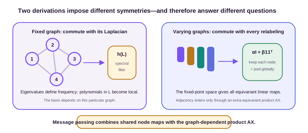
The complete linear characterization for node features appears too restrictive compared with a GNN layer such as \(\mathbf{A}\mathbf{X}\mathbf{W}\). There is no contradiction. The characterization considered a linear map of node features alone. A GNN receives both node features \(\mathbf{X}\) and a graph \(\mathbf{A}\), and the two inputs transform together:

\[\mathbf{X}\mapsto\mathbf{P}\mathbf{X}, \qquad \mathbf{A}\mapsto\mathbf{P}\mathbf{A}\mathbf{P}^{\mathsf T}.\]

Their product is equivariant:

\[(\mathbf{P}\mathbf{A}\mathbf{P}^{\mathsf T})(\mathbf{P}\mathbf{X}) =\mathbf{P}\mathbf{A}\mathbf{X}.\]

The map \((\mathbf{A},\mathbf{X})\mapsto\mathbf{A}\mathbf{X}\) is bilinear, not linear in the pair jointly. It lets the graph choose which nodes communicate without tying the model to their numerical indices. A shared node-wise transformation is also equivariant, and a pointwise nonlinearity preserves equivariance. Their composition gives the basic message-passing pattern.

On the three-node path, \(\mathbf A\mathbf e_1=(0,1,0)^{\mathsf T}\). The adjacency distinguishes node 2 from node 3 even though the impulse features do not. Combining the two equivariant contractions \(\alpha\mathbf x+\beta\mathbf A\mathbf x\) yields \((\alpha,\beta,0)^{\mathsf T}\), which can represent any degree-one endpoint response, including \((3/4,1/4,0)\). The feature-only commutant could not.

Simultaneous relabeling proves the construction rather than merely illustrating it:

\[(\mathbf P\mathbf A\mathbf P^{\mathsf T})(\mathbf P\mathbf X) =\mathbf P\mathbf A(\mathbf P^{\mathsf T}\mathbf P)\mathbf X =\mathbf P(\mathbf A\mathbf X).\]

The order-2 adjacency supplies a relation; the shared contraction supplies equivariance. The message-passing chapter develops the architectural choices that follow—learned messages, attention, aggregation, and controlled model comparisons. Here \(\mathbf A\mathbf X\) marks the exact algebraic bridge between tensor fixed points and a local graph operator.

This explains why permutation symmetry alone cannot discover local neighborhoods. Under the full permutation group, no pair of distinct node indices is privileged. The adjacency matrix supplies the relational structure, and simultaneous relabeling ensures that structure is used consistently. The spectral route encodes the same structure inside \(\mathbf{L}\); the equivariant route keeps it visible as an input.

What the two derivations reveal—and hide

The spectral derivation explains frequency, smoothing, and locality. The Laplacian quadratic form gives frequency a precise meaning. A response \(h(\lambda)\) states which variations the layer preserves. Polynomial approximation explains why a frequency-domain filter can be evaluated through local neighborhoods. This viewpoint also clarifies oversmoothing: repeatedly applying a low-pass operator suppresses high-frequency components and drives node representations toward a low-dimensional smooth subspace.

The same derivation hides several choices. Frequency depends on the selected Laplacian, and combinatorial, symmetric-normalized, and random-walk Laplacians impose different scales. Individual eigenvectors have sign ambiguity, repeated eigenvalues have basis ambiguity, and disconnected graphs have a multidimensional zero-eigenvalue space. Direct spectral parameters are tied to one graph; only structured responses such as polynomials transfer naturally.

The permutation-equivariant derivation explains weight sharing and completeness. It states the symmetry for variable graphs without choosing coordinates or eigenvectors. The fixed-point view can enumerate every linear equivariant map at a given tensor order, making clear which operations are forced by symmetry and which are architectural choices.

Its blind spot is graph geometry. Equivariance to every relabeling says how indices may change, but it does not say which nodes are adjacent or how far apart they are. Without \(\mathbf{A}\), the only linear node operations are self-information and global pooling. Once adjacency enters, useful graph layers become nonlinear or bilinear functions of their full input, and the tidy linear classification no longer describes the whole architecture. At higher tensor orders, the number of equality-pattern bases also grows rapidly, making the complete family expensive.

Message passing occupies the practical middle. It uses permutation-equivariant parameter sharing, lets the adjacency matrix define locality, and learns nonlinear feature transformations around a sparse aggregation. A GCN chooses a particularly simple normalized linear aggregation motivated by a first-order spectral filter. GraphSAGE, GAT, and GIN keep the same symmetry while changing how messages are weighted and combined. The spectral argument explains one member of the family; permutation equivariance explains the family resemblance.

The computational difference is concrete. A dense eigendecomposition costs \(O(N^3)\) time and stores \(O(N^2)\) eigenvectors. Applying a free spectral multiplier then requires two dense transforms, \(O(N^2d)\) for \(d\) channels. A degree-\(K\) polynomial on a sparse graph uses \(K\) sparse matrix products, $$O(K

E

d)\(time and\)O(

E

+Nd)\(working memory. A one-hop GCN aggregation is\)O(

E

d)\(, followed by channel mixing whose dense cost is\)O(Nd_{\mathrm{in}}d_{\mathrm{out}})$$. These counts omit batching and hardware constants, but they explain why localized operators dominate variable-graph learning.

Complete higher-order equivariant maps pay elsewhere. An order-2 feature tensor stores \(O(N^2d)\) values even though its matrix-to-matrix linear basis has only 15 equality patterns in the \(N\ge4\) stable regime. Parameter sharing controls the number of learned coefficients; it does not remove the tensor storage. Sparse graph contractions avoid materializing most pairs by accepting the adjacency-defined support.

The two routes support different claims:

claim	Laplacian–spectral route	permutation–commutant route
basic object	one graph operator \(\mathbf L\)	a group action on indexed inputs
exact guarantee	\(h(\mathbf L)\) is diagonal by eigenspace; polynomials are relabeling equivariant when \(\mathbf L\) and features transform together	enumerated linear maps commute with every relabeling at the stated tensor orders
source of locality	finite polynomial degree	supplied sparse relation such as \(\mathbf A\)
source of frequency	Laplacian quadratic form and spectrum	none from symmetry alone
transfer across graph sizes	only structured responses such as shared polynomial coefficients	built into index sharing, provided relational inputs transform jointly
GCN connection	first-order restriction plus coefficient tying, \(\lambda_{\max}\) approximation, and renormalization	shared feature maps composed with the bilinear contraction \(\mathbf A\mathbf X\)
main blind spot	operator choice and graph-specific spectrum	graph geometry unless supplied as input

The overlap is exact for a shared polynomial of an equivariantly relabeled graph operator: it is simultaneously a spectral response and a permutation-equivariant graph computation. The practical GCN sits nearby, not at the endpoint of an equality chain, because renormalization changes the operator.

The phrase “graph convolution” therefore carries two legitimate meanings. It can mean a function of a graph Laplacian, diagonal in a graph Fourier basis. Or it can mean a translation-inspired equivariant layer on graph-structured data. The first meaning is sharper mathematically but tied to a graph operator. The second travels across graphs but needs the adjacency matrix to say what local structure is. Keeping both meanings visible is more useful than forcing either derivation to do the other’s job.

---

References

1. Shuman, D. I., Narang, S. K., Frossard, P., Ortega, A., & Vandergheynst, P. (2013). The emerging field of signal processing on graphs: Extending high-dimensional data analysis to networks and other irregular domains. IEEE Signal Processing Magazine, 30(3), 83–98. ↩
2. Defferrard, M., Bresson, X., & Vandergheynst, P. (2016). Convolutional neural networks on graphs with fast localized spectral filtering. Advances in Neural Information Processing Systems, 29. ↩
3. Kipf, T. N., & Welling, M. (2017). Semi-supervised classification with graph convolutional networks. International Conference on Learning Representations. ↩
4. Zaheer, M., Kottur, S., Ravanbakhsh, S., Póczos, B., Salakhutdinov, R. R., & Smola, A. J. (2017). Deep Sets. Advances in Neural Information Processing Systems, 30. ↩
5. Maron, H., Ben-Hamu, H., Shamir, N., & Lipman, Y. (2019). Invariant and equivariant graph networks. International Conference on Learning Representations. ↩