What Graph Neural Networks Can and Cannot Distinguish

Adapted from my 2025 Machine Learning for Molecules and Geometric Deep Learning lectures. The useful question is not which graph architecture has the longest feature list, but which distinctions its representation preserves, which it erases, and whether the surviving distinctions matter for the task.

A graph neural network can fail after optimization has done everything right. Two different graphs may receive exactly the same representation for every possible parameter setting. More data, wider hidden states, and longer training cannot recover information that the representation erased before prediction began.

This is an approximation problem, not merely a graph-isomorphism curiosity. A representation partitions graphs into equivalence classes. Every predictor built on top of it must be constant inside each class. If the target is not constant there, the model class has irreducible error. If the target is constant there, making the representation finer may add computation and variance without adding useful signal.

The one-dimensional Weisfeiler–Leman test (1-WL) makes this boundary unusually concrete. It repeatedly replaces each node’s color by an injective code of the node’s current color and the multiset of neighboring colors. Standard message-passing neural networks perform the same kind of local symmetric computation, so 1-WL gives them an architectural ceiling. This post derives that ceiling carefully, then keeps one collision—a six-cycle versus two disjoint triangles—fixed while changing the assumptions behind it. Tuple states, motif counts, bags of subgraphs, and spectral positions all separate the pair, but for different reasons and at different costs.

The architecture of message passing itself is developed in Graph Neural Networks as Learnable Message Passing. Here the question begins one level later: once a network is permutation symmetric, which non-isomorphic inputs must it still identify?

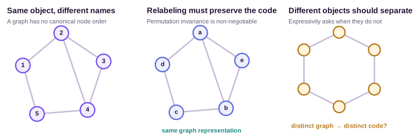
A representation should identify graphs, not node names

Let \(G=(V,E,\mathbf{X})\) be a graph with node set \(V\), edge set \(E\), and node-feature matrix \(\mathbf{X}\). Write \(\mathbf{A}\) for its adjacency matrix. A permutation matrix \(\mathbf{P}\) changes only the storage order:

\[\mathbf{X}'=\mathbf{P}\mathbf{X}, \qquad \mathbf{A}'=\mathbf{P}\mathbf{A}\mathbf{P}^{\mathsf T}.\]

A graph-level representation \(R\) must be invariant to this relabeling,

\[R(\mathbf{P}\mathbf{X},\mathbf{P}\mathbf{A}\mathbf{P}^{\mathsf T}) =R(\mathbf{X},\mathbf{A}),\]

because the node indices are not part of the combinatorial object. Two attributed graphs \(G\) and \(H\) are isomorphic when a bijection \(\varphi:V(G)\to V(H)\) preserves both features and adjacency. Invariance requires isomorphic graphs to share a representation. Expressivity asks how often the converse fails.

Every representation defines a quotient

Fix a graph domain \(\mathcal{G}\) and a deterministic representation \(R:\mathcal{G}\to\mathcal{Z}\). Define

\[G\sim_R H \quad\Longleftrightarrow\quad R(G)=R(H).\]

Equality in \(\mathcal{Z}\) makes \(\sim_R\) an equivalence relation: it is reflexive, symmetric, and transitive. The representation therefore replaces \(\mathcal{G}\) by the quotient \(\mathcal{G}/\!\sim_R\), whose elements are equivalence classes

\[[G]_R=\{H\in\mathcal{G}:R(H)=R(G)\}.\]

An invariant representation must place the entire isomorphism class of \(G\) inside \([G]_R\). A complete invariant would make the two classes equal: \(R(G)=R(H)\) if and only if \(G\cong H\). Most practical representations are coarser. Their classes contain several non-isomorphic graphs.

Now attach a predictor \(g:\mathcal{Z}\to\mathbb{R}\). The composed model \(f=g\circ R\) is necessarily constant on every class \([G]_R\). Suppose two graphs collide but their scalar targets differ:

\[R(G)=R(H), \qquad y(G)\neq y(H).\]

If \(z=R(G)=R(H)\) and \(a=g(z)\), the triangle inequality gives

\[|y(G)-y(H)| \leq |y(G)-a|+|a-y(H)|.\]

At least one error must therefore be half the target gap or larger:

\[\inf_g\max\bigl\{|g(R(G))-y(G)|,|g(R(H))-y(H)|\bigr\} \geq \frac{|y(G)-y(H)|}{2}.\]

This lower bound quantifies the obstruction. It ranges over every downstream function \(g\), so it is unaffected by optimization or network width. Under squared loss on a distribution of graphs, the best prediction based only on \(R(G)\) is the conditional mean \(\mathbb{E}[Y\mid R(G)]\), and its residual risk is

\[\inf_g\mathbb{E}\bigl[(Y-g(R(G)))^2\bigr] =\mathbb{E}\bigl[\operatorname{Var}(Y\mid R(G))\bigr].\]

The same quotient can therefore be adequate for one target and inadequate for another. A degree-sequence representation may be sufficient for a target defined from degrees, while being useless for connectedness. There is no task-independent scalar called “the expressivity” of a representation; there is a relation between its equivalence classes and the target.

The reverse distinction matters just as much. If \(R(G)\neq R(H)\), the architecture can give different outputs, but training may choose parameters that do not. Architectural indistinguishability is universal over parameters. A training failure concerns one fitted parameter value. Confusing the two turns a theorem about a function class into an anecdote about an optimizer.

Message passing compresses a multiset

A message-passing neural network (MPNN) updates node \(v\) from its state and the states of its neighbors. At layer \(t\),

\[\begin{aligned} \mathbf{m}_{v}^{(t)} &=\operatorname{AGG}^{(t)}\!\left( \left\{\!\left\{ M^{(t)}\!\left(\mathbf{h}_{v}^{(t-1)}, \mathbf{h}_{u}^{(t-1)},\mathbf{e}_{uv}\right) :u\in\mathcal{N}(v) \right\}\!\right\}\right),\\ \mathbf{h}_{v}^{(t)} &=U^{(t)}\!\left(\mathbf{h}_{v}^{(t-1)},\mathbf{m}_{v}^{(t)}\right). \end{aligned}\]

The double braces denote a multiset: multiplicities matter, order does not. The aggregator must ignore neighbor order, but order invariance alone does not say which multisets it preserves.

Three elementary collisions

Consider scalar neighbor features. Mean aggregation identifies multisets whose empirical averages match:

\[\operatorname{mean}\{\!\{1,3\}\!\} =2 =\operatorname{mean}\{\!\{1,1,3,3\}\!\}.\]

It has erased a uniform replication of the neighborhood. Maximum aggregation erases multiplicity even when replication is not uniform:

\[\max\{\!\{1,3\}\!\} =3 =\max\{\!\{1,1,3\}\!\}.\]

A raw scalar sum retains those particular multiplicities but is not universally injective:

\[\sum\{\!\{1,3\}\!\} =4 =\sum\{\!\{2,2\}\!\}.\]

The last equation does not say that sum aggregation is no better than mean. It says that injectivity belongs to the encoding followed by the sum, not to addition of arbitrary raw values. A learned map \(\phi\) can encode elements before summation,

\[R(S)=\sum_{x\in S}\phi(x),\]

and, on an appropriate multiset domain, make this map injective.

A bounded-domain injective sum

The finite case makes the claim exact. Suppose each element belongs to \(\{0,1,\ldots,q-1\}\) and every multiset has size at most \(B\). Choose

\[\phi(j)=(B+1)^j.\]

If \(c_j\in\{0,1,\ldots,B\}\) is the multiplicity of symbol \(j\), then

\[\sum_{x\in S}\phi(x) =\sum_{j=0}^{q-1}c_j(B+1)^j.\]

This is the base-\((B+1)\) numeral whose digits are the counts \((c_0,\ldots,c_{q-1})\). Base expansions with digits between \(0\) and \(B\) are unique, so two sums agree only when every multiplicity agrees. The representation is injective on this bounded family. A one-hot map \(\phi(j)=\mathbf{e}_j\in\mathbb{R}^q\) gives the same conclusion more transparently: the sum is simply the count vector.

The assumptions do real work. Without a bound on multiplicity, a fixed base permits carries. Without a discrete or suitably restricted element domain, finite-dimensional continuous encodings need additional conditions. The GIN analysis of Xu et al., 2019 uses the bounded, countable setting to show that a sum followed by a sufficiently expressive multilayer perceptron can represent injective multiset functions. Its update is

\[\mathbf{h}_{v}^{(t)} =\operatorname{MLP}^{(t)}\!\left( (1+\epsilon^{(t)})\mathbf{h}_{v}^{(t-1)} +\sum_{u\in\mathcal{N}(v)}\mathbf{h}_{u}^{(t-1)} \right).\]

The coefficient \(1+\epsilon^{(t)}\) helps keep the center separate from the neighbor multiset. Injectivity prevents avoidable collisions inside one aggregation step. It does not reveal structures that every node-centered multiset computation sees as identical. That remaining limit is exactly what 1-WL describes.

Color refinement is the discrete analogue

The one-dimensional Weisfeiler–Leman test, usually called 1-WL or color refinement, replaces learned vectors by discrete colors. Begin with an initial color \(c_v^{(0)}\) for every node. At iteration \(t\), form the signature

\[s_v^{(t)} =\left(c_v^{(t-1)}, \left\{\!\left\{c_u^{(t-1)}:u\in\mathcal{N}(v)\right\}\!\right\}\right)\]

and assign

\[c_v^{(t)}=\operatorname{HASH}\!\left(s_v^{(t)}\right),\]

where \(\operatorname{HASH}\) is injective on the signatures that occur. Two graphs are refined jointly, so the same signature receives the same color name in both. If their color histograms differ at any round, they cannot be isomorphic. If the histograms remain equal after stabilization, 1-WL returns “not distinguished,” not “isomorphic.” The procedure goes back to Weisfeiler and Leman, 1968.

Every signature on the five-node path

Let \(P_5\) have vertices \(v_1-v_2-v_3-v_4-v_5\), and initialize every vertex with color \(a\). At round zero,

\[(c_{v_1}^{(0)},c_{v_2}^{(0)},c_{v_3}^{(0)},c_{v_4}^{(0)},c_{v_5}^{(0)}) =(a,a,a,a,a).\]

At round one, the endpoints have one neighbor and the other vertices have two:

\[\begin{array}{c|c|c} \text{vertices} & \text{signature} & \text{new color}\\ \hline v_1,v_5 & (a,\{\!\{a\}\!\}) & b\\ v_2,v_3,v_4 & (a,\{\!\{a,a\}\!\}) & c. \end{array}\]

Thus the ordered color sequence is \((b,c,c,c,b)\). Degree was enough for this first split, but degree no longer explains round two. The three internal vertices now see different colored neighborhoods:

\[\begin{array}{c|c|c} \text{vertices} & \text{signature} & \text{new color}\\ \hline v_1,v_5 & (b,\{\!\{c\}\!\}) & d\\ v_2,v_4 & (c,\{\!\{b,c\}\!\}) & e\\ v_3 & (c,\{\!\{c,c\}\!\}) & f. \end{array}\]

The sequence becomes \((d,e,f,e,d)\). At round three the signatures are

\[\begin{aligned} v_1,v_5 &: (d,\{\!\{e\}\!\}),\\ v_2,v_4 &: (e,\{\!\{d,f\}\!\}),\\ v_3 &: (f,\{\!\{e,e\}\!\}). \end{aligned}\]

They receive new names, but the partition into three cells does not refine further. This is the stable coloring. The equality of \(v_1\) with \(v_5\) and of \(v_2\) with \(v_4\) is not a weakness: the path has a reflection automorphism exchanging those pairs, so any isomorphism-respecting node representation must identify them. The singleton center occupies its own orbit.

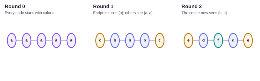
Color names have no numerical meaning. Color \(f\) is not larger than color \(e\); it is a lossless name for one signature. After \(t\) rounds, a color records the rooted, unfolded neighborhood pattern visible through \(t\) rounds of refinement. Cycles and repeated vertices in the original graph are not necessarily recorded faithfully in that unfolding, which is where collisions enter.

Standard MPNNs inherit the 1-WL ceiling

We can now state the ceiling without hiding its quantifiers.

The 1-WL ceiling for graph-level message passing. Let \(G\) and \(H\) be finite attributed graphs. Run 1-WL jointly on their node and edge labels, using an injective hash of the center color and the multiset of labeled neighbor colors. Consider any depth \(T\geq0\) and any deterministic MPNN whose initial state is a shared function of the initial node label, whose edge messages and node updates are shared across the graph, whose neighborhood aggregation is permutation invariant, and whose graph readout is permutation invariant. If the two graphs have the same 1-WL color histogram at every round \(t=0,\ldots,T\), then for every choice of the MPNN’s functions and parameters their graph outputs after \(T\) layers are equal.

The statement is universal over depth, functions, and parameter values once the assumptions are fixed. It is not a claim about a trained checkpoint. It also allows arbitrary hidden width and nonlinear message functions.

Proof by induction on color classes

We prove the stronger node statement: for every layer \(t\leq T\), there exists a function \(\psi_t\) such that

\[\mathbf{h}_v^{(t)}=\psi_t(c_v^{(t)})\]

for every node of either graph. Equivalently, equal 1-WL colors imply equal hidden states.

At \(t=0\), the claim holds because initialization is a shared function of the initial label. Assume it holds at \(t-1\). If \(c_v^{(t)}=c_w^{(t)}\), injectivity of the WL hash implies two facts:

1. \(c_v^{(t-1)}=c_w^{(t-1)}\).
2. The multisets of labeled neighbor colors around \(v\) and \(w\) are equal.

By the induction hypothesis, the center states are equal. Applying \(\psi_{t-1}\) to equal neighbor-color multisets gives equal multisets of neighbor states, with edge-label correspondence included when edges are attributed. The shared message function maps corresponding entries to equal messages. Permutation-invariant aggregation maps the equal message multisets to the same aggregate, and the shared update maps equal center-state/aggregate pairs to equal new states. Thus equal round-\(t\) colors imply equal layer-\(t\) states.

If \(G\) and \(H\) have the same color histogram at round \(T\), each color occurs with the same multiplicity in both. Since hidden state is a function of color, their multisets of final hidden states are equal. A permutation-invariant readout must return the same graph representation, and any shared downstream predictor returns the same output. This completes the proof.

Morris et al., 2019 and Xu et al. established closely related neural versions of the WL correspondence. The converse requires stronger assumptions: when aggregation, update, and readout are injective on the relevant bounded domains, an MPNN can match 1-WL’s distinctions. GIN is a constructive route to that matching case. A mean-based or otherwise non-injective MPNN may be strictly weaker than 1-WL.

Three boundaries of the theorem are worth making explicit. First, it is a one-way ceiling: 1-WL equivalence forces MPNN equivalence, but 1-WL distinction does not force every parameterized MPNN to distinguish. Second, informative continuous attributes may separate graphs that collide when unlabeled; then 1-WL and the MPNN operate on a different, enriched input. Third, unique identifiers can destroy the collision, but fixed arbitrary IDs also destroy the intended invariance unless the model treats their randomness or permutation carefully.

A six-cycle looks like two triangles

Let \(G=C_6\) be a cycle on six vertices and let \(H=2C_3\) be the disjoint union of two triangles. They are not isomorphic. The first is connected and has no triangles; the second has two connected components and two triangles. Yet both are 2-regular.

Initialize every node with the same color \(a_0\). Suppose at round \(t\) every node in both graphs has color \(a_t\). Every node has exactly two neighbors, both colored \(a_t\), so every signature is

\[(a_t,\{\!\{a_t,a_t\}\!\}).\]

The joint injective hash assigns all twelve nodes the same next color \(a_{t+1}\). Induction shows that at every round, each graph’s histogram contains six copies of one common color. Therefore 1-WL never distinguishes them.

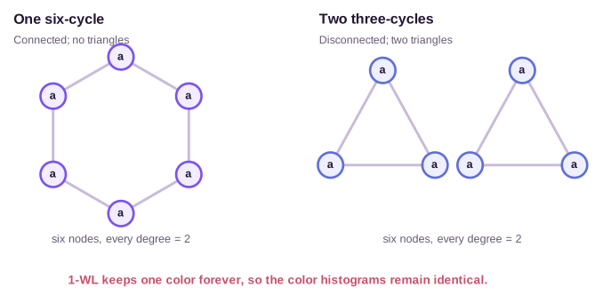
The ceiling theorem converts that discrete calculation into a neural impossibility statement. For every standard MPNN satisfying the theorem, for every parameter setting, and for every depth, uniform initial features produce the same graph output on \(C_6\) and \(2C_3\). This is stronger than saying six layers are insufficient. The refinement has reached a fixed point after its first update; extra layers repeat the collision.

The target obstruction is now numerical. Define \(y_{\triangle}(G)\) as the number of undirected triangles. Then

\[y_{\triangle}(C_6)=0, \qquad y_{\triangle}(2C_3)=2.\]

Any scalar predictor built on the colliding representation has worst-case absolute error at least \(1\) on this pair. The best common prediction under equal weighting is \(1\). For the connectedness indicator \(y_{\mathrm{conn}}\), the values are \(1\) and \(0\), so the corresponding lower bound is \(1/2\).

This witness is deliberately small, but it isolates the mechanism. Real molecular graphs often have atom and bond labels that destroy uniformity. That does not invalidate the theorem; it changes the initial colors. Expressivity claims should always name the input attributes under which a collision holds.

Stronger models change what gets compared

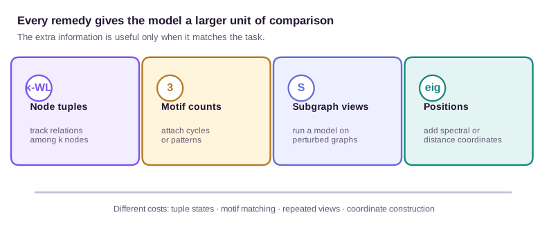
Going beyond the ceiling means changing at least one theorem assumption. A deeper MLP inside the same node-wise update does not. The four remedies below all revisit \(C_6\) versus \(2C_3\) so that the source of each new distinction remains visible.

Compare tuples instead of individual nodes

Higher-order WL stores colors on ordered tuples rather than individual nodes. There is a nomenclature trap here. The coordinate-wise algorithm commonly called \(2\)-WL aggregates replacements of the first and second coordinate in separate multisets. The folklore \(2\)-WL algorithm, abbreviated \(2\)-FWL, keeps the two replacements associated with the same intermediate vertex. For an ordered pair \((u,v)\), initialize a color \(c_{uv}^{(0)}\) that records whether \(u=v\), whether \(u\) and \(v\) are adjacent, and their attributes. Its joint replacement multiset is

\[\mathcal{M}_{uv}^{(t)} =\left\{\!\left\{ \left(c_{uw}^{(t-1)},c_{wv}^{(t-1)}\right):w\in V \right\}\!\right\}.\]

The update injectively encodes \((c_{uv}^{(t-1)},\mathcal{M}_{uv}^{(t)})\). This precise relational pair refinement—not the weaker coordinate-wise convention—is what the common-neighbor calculation below uses. In distinguishing power, \(2\)-FWL corresponds to \(3\)-WL; the matrix-multiplication network of Maron et al., 2019 realizes this stronger pair interaction with second-order states.

Take an adjacent ordered pair \((u,v)\). In \(C_6\), no vertex is adjacent to both endpoints of an edge, so

\[\bigl|\mathcal{N}(u)\cap\mathcal{N}(v)\bigr|=0.\]

In \(2C_3\), every edge belongs to exactly one triangle, and its third vertex is a common neighbor:

\[\bigl|\mathcal{N}(u)\cap\mathcal{N}(v)\bigr|=1.\]

Consequently \(\mathcal{M}_{uv}^{(1)}\) contains zero \((\text{edge},\text{edge})\) entries for an edge of \(C_6\) and one for an edge of \(2C_3\). Folklore \(2\)-WL therefore separates their edge-pair colors after one update, and the graph histograms then differ. More generally, higher-order GNNs translate tuple refinements into neural states; Morris et al. give a hierarchy tied to the coordinate-wise higher-order WL construction, while Maron et al. show how a quadratic pair-state operation reaches the stronger \(3\)-WL, or \(2\)-FWL, distinction used here.

The changed assumption is precise: hidden states now live on ordered pairs, not only on nodes. There are \(n^2\) pair states instead of \(n\) node states. With width \(d\), dense pair storage is \(O(n^2d)\). Aggregating over all replacement vertices for every pair is \(O(n^3d)\) per layer before channel transformations, compared with roughly \(O(md)\) aggregation for a sparse node MPNN with \(m\) directed message edges. A general \(k\)-tuple construction has \(O(n^kd)\) state; dense replacement refinement adds another factor of \(n\). Local and sparse variants reduce this cost by restricting tuples, which also changes the exact guarantee.

Expose selected substructures

A motif encoding keeps node states but augments their input with a statistic that node-wise 1-WL could not derive. For triangles, the adjacency identity is

\[N_{\triangle}(G)=\frac{1}{6}\operatorname{tr}(\mathbf{A}^3).\]

Each triangle contributes six oriented closed walks of length three: three starting vertices times two directions. A six-cycle has no length-three closed walk, so \(\operatorname{tr}(\mathbf{A}_{C_6}^3)=0\). Two triangles contribute twelve, so

\[\frac{1}{6}\operatorname{tr}(\mathbf{A}_{2C_3}^3)=2.\]

Equivalently, attach to each node the number of triangles containing it. Every node of \(C_6\) receives \(0\) and every node of \(2C_3\) receives \(1\). Even a zero-layer sum readout then distinguishes the graphs: the augmented coordinate sums to \(0\) versus \(6\).

Graph Substructure Networks make this strategy systematic by supplying subgraph-isomorphism counts to message passing (Bouritsas et al., 2021). The theorem assumption that changed is initial information. The downstream network may still be an ordinary node MPNN, but it no longer receives only the original unlabeled graph.

The cost is paid in motif selection and preprocessing. Dense multiplication computes \(\operatorname{tr}(\mathbf{A}^3)\) in cubic time by the elementary algorithm, although triangle-specific sparse algorithms can exploit adjacency intersections. A direct node-centered procedure costs on the order of \(\sum_v d_v^2\) membership checks before data-structure effects, which is much smaller on many sparse graphs but large around hubs. Counting arbitrary motifs is harder, and a finite motif bank only separates graphs along chosen axes. Triangle counts solve this witness because the target distinction was built around triangles; they do not form a universal complete invariant.

Represent the graph through a bag of subgraphs

Subgraph GNNs change the input from one graph to an invariant bag of related views. Delete one vertex from each graph and examine the resulting six-card deletion deck.

Deleting any vertex from \(C_6\) produces the five-node path \(P_5\). Deleting a vertex from \(2C_3\) leaves one intact triangle and one edge, \(C_3\sqcup K_2\). Both cards have degree multiset

\[\{\!\{1,1,2,2,2\}\!\},\]

so degree alone still collides. One further 1-WL round separates them. In \(P_5\), each degree-one endpoint is adjacent to a degree-two vertex. In \(C_3\sqcup K_2\), each degree-one vertex is adjacent to the other degree-one vertex. Their endpoint signatures are respectively

\[(1,\{\!\{2\}\!\}) \qquad\text{and}\qquad (1,\{\!\{1\}\!\}).\]

Thus a 1-WL-powered base network can distinguish every card of the first deck from every card of the second. The invariant bag contains six copies of \(P_5\) for \(C_6\) and six copies of \(C_3\sqcup K_2\) for \(2C_3\). Aggregating card representations separates the original graphs.

Equivariant Subgraph Aggregation Networks formalize the nested symmetry: node order within each view and view order within the bag are both arbitrary (Bevilacqua et al., 2022). The changed assumption is that the model observes a family of interventions on the graph, not only node-centered neighborhoods in the original graph.

Exhaustive one-node deletion creates \(n\) views, each with \(n-1\) nodes and at most \(m\) edges. Storing all view-level node states costs \(O(n^2d)\), and running a sparse \(T\)-layer base MPNN independently costs roughly \(O(Tnmd)\) for aggregation, ignoring feature transforms and the few deleted edges. Sampling views lowers the multiplier but can miss a decisive card and replaces an exhaustive invariance statement by a stochastic approximation. Marking rather than deleting nodes changes the deck again; the selection policy is part of the representation, not an implementation detail.

Supply structural positions

Spectral information offers a global coordinate system derived from the graph. Let \(\mathbf{L}=\mathbf{D}-\mathbf{A}\) be the combinatorial Laplacian. The eigenvalues of a cycle are

\[\lambda_k(C_n)=2-2\cos\!\left(\frac{2\pi k}{n}\right), \qquad k=0,\ldots,n-1.\]

For \(C_6\) this gives

\[\operatorname{spec}(\mathbf{L}_{C_6}) =\{\!\{0,1,1,3,3,4\}\!\}.\]

A triangle has spectrum \(\{\!\{0,3,3\}\!\}\), and the Laplacian of a disjoint union is block diagonal, so

\[\operatorname{spec}(\mathbf{L}_{2C_3}) =\{\!\{0,0,3,3,3,3\}\!\}.\]

The multiplicity of eigenvalue zero equals the number of connected components, making the distinction immediate. A graph-level spectrum feature separates the pair without message passing. Node-wise Laplacian eigenvectors or pairwise shortest-path encodings can likewise expose global position to a Transformer or MPNN.

The changed assumption is again the input information, but now the added statistic is global rather than a selected local motif. The price is numerical and conceptual. A dense eigendecomposition costs \(O(n^3)\) time and \(O(n^2)\) storage. Keeping \(k\) eigenvectors uses \(O(nk)\) feature storage, while iterative sparse eigensolvers can exploit matrix-vector products costing \(O(mk)\) per iteration; their total cost depends on spectral gaps and convergence, so \(O(mk)\) is not a complete runtime claim.

Eigenvectors are also coordinates without a unique frame. A simple eigenvector may flip sign, and a repeated eigenspace may rotate by any orthogonal basis change. Here \(C_6\) has repeated eigenvalues \(1\) and \(3\), so raw basis vectors are especially non-canonical. SignNet and BasisNet construct functions invariant to these ambiguities (Lim et al., 2023). Spectrum-only methods avoid basis choice but are not complete: non-isomorphic cospectral graphs exist. Structural positions exchange the 1-WL collision for a different quotient and a different set of ambiguities.

Random identifiers illustrate the same principle more sharply. Independent node IDs almost surely break the uniform coloring, but fixed IDs tie outputs to arbitrary names. Averaging predictions over fresh random IDs can recover invariance in expectation, with Monte Carlo variance and repeated evaluation. The apparent expressivity did not come from a better local aggregator; it came from additional symmetry-breaking information plus a procedure for restoring the desired symmetry.

The controlled comparison

The same witness now exposes four distinct changes:

representation	exact separator on \(C_6\) vs. \(2C_3\)	assumption changed	leading state / work
node MPNN / 1-WL	none from uniform labels	baseline node-centered multisets	\(O(nd)\) state; about \(O(md)\) aggregation per layer
folklore \(2\)-WL pair refinement	common neighbors of an edge: \(0\) vs. \(1\)	states live on ordered pairs with joint replacements	\(O(n^2d)\) state; dense \(O(n^3d)\) refinement
triangle features	\(\operatorname{tr}(\mathbf{A}^3)/6=0\) vs. \(2\)	motif counts enter the input	preprocessing; dense cubic or motif-specific sparse counting
deletion-view bag	six \(P_5\) cards vs. six \(C_3\sqcup K_2\) cards	model observes graph interventions	\(O(n^2d)\) view state; roughly \(n\) base-network runs
Laplacian features	spectra \(\{\!\{0,1,1,3,3,4\}\!\}\) vs. \(\{\!\{0,0,3,3,3,3\}\!\}\)	global structural coordinates enter	dense \(O(n^3)\) solve; \(O(nk)\) retained coordinates

These are not interchangeable implementations of one abstract “more expressive GNN.” Pair states derive a relation internally by enlarging the state space. Motif encodings supply a chosen answer in advance. Deletion bags evaluate counterfactual views. Spectral methods supply a global coordinate system. Each creates a finer quotient of graph space, but the new equivalence classes need not be nested in exactly the same way outside this example.

Expressivity is not model quality

The quotient view gives a clean stopping rule. A target \(y\) factors through representation \(R\) precisely when there exists some \(g\) such that

\[y=g\circ R.\]

Equivalently,

\[G\sim_R H \quad\Longrightarrow\quad y(G)=y(H).\]

When this condition holds, the representation creates no information-theoretic obstruction for that target, even if it fails many graph-isomorphism tests. When it fails, no downstream learner can repair the collision. Expressivity matters through this target-relative condition, not through a leaderboard of increasingly fine graph invariants.

When separating more graphs helps

On our witness, added distinctions are essential for triangle count, connectedness, girth, and any target assigning different values to the two graphs. A triangle feature is a particularly efficient bias when the scientific target depends on three-membered rings. Pair states may be preferable when many relational motifs matter and preselecting a motif bank would be brittle. Deletion views are attractive when response to local removal is itself meaningful, as in robustness or influence problems. Spectral features are natural for diffusion, connectivity, and low-frequency global organization.

The target gap tells us the minimum price of ignoring the distinction. For triangle count, the common-output absolute-error lower bound is \(1\). For a binary connectedness label it is \(1/2\). If the two graphs occur with probabilities \(p\) and \(1-p\) and the target is connectedness, the optimal common squared-loss prediction is \(p\), with risk \(p(1-p)\). Better optimization cannot push below that conditional variance; a representation that separates the pair can, in principle, reduce it to zero.

Distinctions can also support transfer when they align with stable mechanisms. Counting a chemically meaningful motif is more likely to transfer than memorizing a graph ID if the motif participates causally in the property. A global position can help a routing model because path length remains meaningful across graph sizes. Expressivity is valuable when its new coordinates match regularities shared by training and deployment graphs.

When separating more graphs hurts

Suppose instead that $$y(G)=

V(G)

\(. Both witness graphs have target\)6\(, and a sum readout can recover size without separating their topology. Or suppose the target is constant on all 2-regular six-node graphs. Refining\)C_6\(away from\)2C_3$$ adds no necessary signal. With finite data, the finer model can fit accidental correlations between triangle structure and noise, increasing estimation error even though approximation error weakly decreases.

The choice can hurt through stability as well. A small graph perturbation can rotate nearly degenerate spectral eigenspaces dramatically even when the underlying target varies smoothly. A sign- and basis-aware architecture repairs formal ambiguity, but it does not eliminate sensitivity caused by a small spectral gap. Unique or random IDs separate nodes maximally while offering little reason for the learned distinction to transfer. A large motif bank can turn rare substructures into high-variance features. Exhaustive deletion bags may spend most computation distinguishing counterfactuals irrelevant to the prediction.

This is the familiar bias–variance tradeoff expressed at the representation level. A coarser quotient imposes bias by forcing several graphs to share a prediction. A finer quotient removes some of that bias but leaves fewer examples per effective class and usually costs more to compute. Neither direction dominates without a data distribution and a target.

Choose the cheapest missing distinction

For a graph with \(n\) nodes, \(m\) directed message edges, hidden width \(d\), and \(T\) layers, ordinary sparse message passing stores \(O(nd)\) node states and spends about \(O(Tmd)\) on aggregation, plus feature transformations. Pair states increase storage to \(O(n^2d)\) and dense refinement to cubic work. Deletion bags multiply a base-network evaluation by roughly \(n\). Spectral coordinates introduce an eigensolve and ambiguity handling. Motif features move computation into a preprocessing algorithm whose scaling depends strongly on the motif and sparsity.

Those costs should buy a named distinction. If connectedness is the only missing signal, a component-count feature may be cheaper and more stable than a full pair network. If a range of small cycles matters, learned tuple or subgraph machinery may justify its broader state. If long-range diffusion modes matter, spectral information may align better than an arbitrary motif bank. There is no virtue in paying \(O(n^3)\) merely to say that a model sits higher in an expressivity hierarchy.

The practical sequence is therefore:

1. Specify the input attributes and the symmetry they must obey.
2. Find graph pairs that the current representation identifies.
3. Ask whether the target separates those pairs, and by how much.
4. Add the cheapest stable statistic or state expansion that exposes the needed difference.
5. Recheck computation, invariance, sample complexity, and out-of-distribution behavior.

The WL hierarchy is useful because it makes step two falsifiable. It turns the vague claim that a GNN “captures structure” into an equivalence relation that can be probed with witnesses and proved with induction. But WL power is not the final objective. A representation is good when it forgets arbitrary node names, retains the distinctions the target needs, and declines to memorize distinctions that the data cannot justify.

---

References

• Weisfeiler, B., & Leman, A. (1968). The reduction of a graph to canonical form and the algebra which appears therein. Nauchno-Technicheskaya Informatsia, 2(9), 12–16. English translation. ↩
• Xu, K., Hu, W., Leskovec, J., & Jegelka, S. (2019). How Powerful Are Graph Neural Networks? ICLR 2019. OpenReview. ↩
• Morris, C., Ritzert, M., Fey, M., Hamilton, W. L., Lenssen, J. E., Rattan, G., & Grohe, M. (2019). Weisfeiler and Leman Go Neural: Higher-order Graph Neural Networks. AAAI 2019. AAAI proceedings. ↩
• Maron, H., Ben-Hamu, H., Serviansky, H., & Lipman, Y. (2019). Provably Powerful Graph Networks. NeurIPS 2019. Proceedings. ↩
• Bouritsas, G., Frasca, F., Zafeiriou, S., & Bronstein, M. M. (2021). Improving Graph Neural Network Expressivity via Subgraph Isomorphism Counting. ICLR 2021. OpenReview. ↩
• Bevilacqua, B., Frasca, F., Lim, D., Srinivasan, B., Cai, C., Balamurugan, G., Bronstein, M. M., & Maron, H. (2022). Equivariant Subgraph Aggregation Networks. ICLR 2022. OpenReview. ↩
• Lim, D., Robinson, J. D., Zhao, L., Smidt, T., Sra, S., Maron, H., & Jegelka, S. (2023). Sign and Basis Invariant Networks for Spectral Graph Representation Learning. ICLR 2023. OpenReview. ↩