Depth, Over-Smoothing, and Over-Squashing in Graph Networks

Adapted from my 2025 Machine Learning for Molecules and Geometric Deep Learning lectures. Starting from message passing, this article asks why information disappears or bottlenecks as graph networks become deep; the expressivity chapter treats the complementary question of which graphs they can distinguish.

A message-passing graph neural network communicates one edge per layer. Two nodes separated by ten edges cannot interact through a five-layer network. The obvious response is to add depth.

Depth solves this reach problem and exposes two harder failures. Repeated propagation can make node representations indistinguishable, which is called over-smoothing. Long-range signals can also be compressed through fixed-width states and narrow graph cuts, which is called over-squashing. These failures are not synonyms. One removes contrast by mixing too much; the other loses sensitivity because too much information must cross too little capacity.

The distinction changes how we design a remedy. Residual connections can preserve local features but leave a topological bottleneck untouched. Rewiring can shorten long paths but accelerate unwanted smoothing. A wider network can carry more information but increase parameters and sensitivity. Deeper graph learning is therefore not a contest to stack the most layers. It is a problem of matching communication range, feature dynamics, and graph topology to the dependency structure of the task.

Depth sets the communication radius

Let \(\mathbf{h}_v^{(\ell)} \in \mathbb{R}^d\) denote the state of node \(v\) after layer \(\ell\). A message-passing layer has the form

\[\mathbf{m}_v^{(\ell)} = \operatorname{AGG} \left\{ M_\ell\!\left( \mathbf{h}_v^{(\ell)}, \mathbf{h}_u^{(\ell)}, \mathbf{e}_{uv} \right) : u \in \mathcal{N}(v) \right\},\] \[\mathbf{h}_v^{(\ell+1)} = U_\ell\!\left( \mathbf{h}_v^{(\ell)}, \mathbf{m}_v^{(\ell)} \right).\]

Here, \(M_\ell\) constructs a message across edge \((u,v)\), \(\operatorname{AGG}\) combines the unordered incoming messages, and \(U_\ell\) updates the receiving node. One layer can only use one-hop neighbors. By induction, \(\mathbf{h}_v^{(L)}\) can depend only on nodes at graph distance at most \(L\) from \(v\).

This \(L\)-hop neighborhood is the model’s receptive field at node \(v\). The term comes from vision, where stacking local convolutions expands the region of an image that can influence one output pixel. On a graph, the receptive field depends on topology. It grows linearly on a path, quadratically on a two-dimensional grid, and exponentially with depth on a regular tree until it reaches the graph boundary.

Insufficient depth causes under-reaching: the target depends on a node outside the receptive field. Consider a molecular bond graph. A two-layer model can couple an atom to atoms at most two bonds away. It cannot directly represent a property whose relevant dependency spans a longer conjugated path. The same issue appears in algorithmic tasks where a node must know whether a distant marked node exists.

An exact depth requirement

Under-reaching is the easiest failure to prove because it follows from locality alone. Take the seven-node path

\[v_0 - v_1 - v_2 - v_3 - v_4 - v_5 - v_6,\]

and place a binary feature \(x_6\in\{0,1\}\) at the right endpoint. The task is to predict \(y_0=x_6\) at the left endpoint. All other node and edge features are identical in the two inputs. A message-passing network with \(L<6\) produces exactly the same state at \(v_0\) whether \(x_6=0\) or \(x_6=1\). Its computation at \(v_0\) only sees \(\{v_0,\ldots,v_L\}\), which is identical in both cases. This statement holds for every width, every parameter choice, and every nonlinear message function that respects the local update above.

At \(L=6\), a computational path from \(v_6\) to \(v_0\) first exists. Six layers are therefore necessary, although not sufficient, for this task. A sum-based construction shows sufficiency in the noiseless toy case: initialize \(h_v^{(0)}=x_v\) and let each node forward the signal from its right neighbor. After six layers, \(h_{v_0}^{(6)}=x_6\). A symmetric aggregator cannot use the phrase “right neighbor” without positional information, but the necessity result does not depend on this construction. It only depends on distance.

The distinction between necessary and sufficient depth is where the other two failure modes enter. Six layers create a route. The product of six propagation operators determines whether the bit arrives with usable magnitude, and the graph’s branching determines how many other bits compete for the same state.

Adding layers expands the receptive field, but reachability only says that a signal can arrive. It does not say that the signal remains identifiable or influential when it does. The three resulting regimes are shown below.

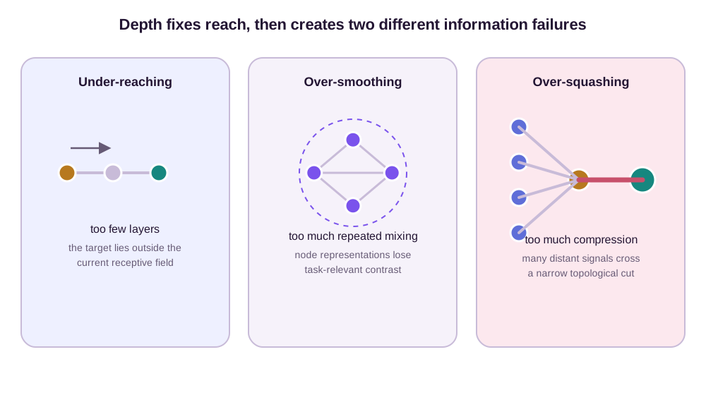
Under-reaching has a direct architectural fix: increase communication range. Over-smoothing and over-squashing require us to ask what happens inside that larger receptive field.

Over-smoothing is a diffusion toward low-frequency features

Many graph layers combine a node with an average of its neighbors. Repeating this operation resembles diffusion: local differences shrink, and the feature field becomes smoother across edges. This is useful when adjacent nodes should have similar representations. It becomes over-smoothing when the diffusion erases distinctions required by the target.

A linear graph convolution makes the mechanism explicit. Add self-loops to the adjacency matrix \(\mathbf{A}\) and call the result \(\widetilde{\mathbf{A}} = \mathbf{A}+\mathbf{I}\). Let \(\widetilde{\mathbf{D}}\) be its degree matrix. The normalized propagation matrix is

\[\mathbf{S} = \widetilde{\mathbf{D}}^{-1/2} \widetilde{\mathbf{A}} \widetilde{\mathbf{D}}^{-1/2}.\]

If we temporarily remove learned weights and nonlinearities, an \(L\)-layer network reduces to

\[\mathbf{H}^{(L)} = \mathbf{S}^L\mathbf{H}^{(0)}.\]

Because \(\mathbf{S}\) is symmetric, it has an orthonormal eigenbasis:

\[\mathbf{S} = \mathbf{U}\boldsymbol{\Lambda}\mathbf{U}^{\mathsf{T}}.\]

The propagated features become

\[\mathbf{H}^{(L)} = \mathbf{U}\boldsymbol{\Lambda}^{L} \mathbf{U}^{\mathsf{T}}\mathbf{H}^{(0)}.\]

Each eigenvector is a graph-frequency pattern, and its coefficient is multiplied by \(\lambda_k^L\). Components with \(\lvert\lambda_k\rvert < 1\) decay geometrically with depth. The dominant low-frequency components survive, so neighboring node features become increasingly aligned. Under conditions on the graph spectrum and layer weights, Oono and Suzuki (2020) formalize an exponential approach toward a low-dimensional subspace that mainly retains connected-component and degree information (Oono & Suzuki, 2020).

This spectral statement has a clean limiting case. For a connected graph with a lazy averaging operator, the largest eigenvalue is \(1\) and all other eigenvalues have magnitude below \(1\). Write one feature channel as

\[\mathbf{x}^{(0)}=c_1\mathbf{u}_1+\sum_{k=2}^{n}c_k\mathbf{u}_k,\]

where \(\mathbf{u}_1\) is the stationary mode. Then

\[\mathbf{x}^{(L)} =c_1\mathbf{u}_1+\sum_{k=2}^{n}c_k\lambda_k^L\mathbf{u}_k \longrightarrow c_1\mathbf{u}_1.\]

The convergence is an exact identity for the linear propagation model, followed by a limit. Calling the same limit “what every trained GNN does” would be an approximation: nonlinearities and learned channel mixing change the operator at every layer. The linear calculation remains useful because it isolates propagation from optimization.

Four nodes make the decay visible

Consider the cycle \(C_4\) and the lazy random-walk propagation

\[\mathbf{S}=\frac{1}{2}\mathbf{I}+\frac{1}{4}\mathbf{A}.\]

Each node keeps half of its value and receives one quarter from each of its two neighbors. The eigenvalues of \(\mathbf{S}\) are \(1,1/2,1/2,0\). Start from the alternating-across-axis feature

\[\mathbf{x}^{(0)}=(1,0,-1,0)^{\mathsf T}.\]

This vector lies in an eigenmode with eigenvalue \(1/2\), so every propagation step halves it:

\[\mathbf{x}^{(1)}=(1/2,0,-1/2,0)^{\mathsf T},\qquad \mathbf{x}^{(2)}=(1/4,0,-1/4,0)^{\mathsf T}.\]

For a scalar feature, the Dirichlet energy below is the sum of squared differences over undirected edges. The four edge differences initially have magnitude one, giving \(\mathcal{E}(\mathbf{x}^{(0)})=4\). They halve after one layer, so the energy quarters:

\[\mathcal{E}(\mathbf{x}^{(L)}) =4\left(\frac{1}{2}\right)^{2L}.\]

The first three energies are therefore \(4,1,1/4\). The feature contrast decays like the eigenvalue to power \(L\), while the quadratic energy decays like its square to power \(L\). This difference matters when reading layerwise plots: a tenfold drop in energy corresponds to only about a threefold drop in feature amplitude.

The same behavior can be measured without diagonalizing \(\mathbf{S}\). Let \(\mathbf{L}=\mathbf{D}-\mathbf{A}\) be the combinatorial graph Laplacian. The Dirichlet energy

\[\mathcal{E}(\mathbf{H}) = \operatorname{tr} \left( \mathbf{H}^{\mathsf{T}}\mathbf{L}\mathbf{H} \right) = \frac{1}{2} \sum_{u\in V} \sum_{v\in\mathcal{N}(u)} \left\lVert \mathbf{h}_u-\mathbf{h}_v \right\rVert_2^2\]

measures variation across edges. Low energy means adjacent features are similar. In the toy linear diffusion above, repeated propagation suppresses feature variation and drives the energy down.

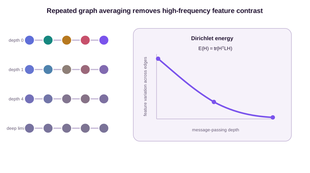
Real GNNs include learned weights, nonlinearities, normalization, and attention, so their Dirichlet energy need not decrease monotonically. Over-smoothing is still the right diagnosis when deeper representations lose node-level separation because propagation repeatedly favors low-frequency structure. It is not the right diagnosis for every failure of a deep model. Optimization can fail while node features remain distinct, and a task can fail because distant signals never arrive even when local features remain sharp.

The spectral gap sets the mixing rate. If \(\rho=\max_{k\geq 2}\lvert\lambda_k\rvert\), the non-stationary component obeys

\[\left\lVert \mathbf{x}^{(L)}-c_1\mathbf{u}_1\right\rVert_2 \leq \rho^L \left\lVert \mathbf{x}^{(0)}-c_1\mathbf{u}_1\right\rVert_2.\]

This is an exact bound for a fixed symmetric propagation matrix. A larger spectral gap \(1-\rho\) means faster mixing and hence faster loss of node contrast. The same gap can be desirable when the target is a slowly varying graph signal. Over-smoothing is not simply “a large gap is bad”; it is a mismatch between the frequencies preserved by propagation and those required by the prediction.

Over-smoothing is also task-dependent. In a homophilic citation graph, papers connected by citations often share a topic, so smoothing can remove noise. In a heterophilic graph, an edge may connect unlike classes, and the same diffusion mixes evidence that should stay separate. A low Dirichlet energy is therefore a geometric statistic, not a certificate of a useful representation.

Residual paths preserve multiple neighborhood scales

The most reliable anti-smoothing methods give a node access to less-propagated features. A residual layer keeps the previous state:

\[\mathbf{H}^{(\ell+1)} = \mathbf{H}^{(\ell)} + F_\ell\!\left(\mathbf{H}^{(\ell)},G\right).\]

The identity path helps optimization and lets information bypass one smoothing step. A residual connection does not remove diffusion from \(F_\ell\), however. Repeated residual layers can still drift toward smooth representations.

Three remedies as graph filters

To compare remedies rather than list them, keep the \(C_4\) input and propagation matrix from the previous section fixed. Use a convex residual update

\[\mathbf{x}^{(\ell+1)} = \alpha\mathbf{x}^{(\ell)} +(1-\alpha)\mathbf{S}\mathbf{x}^{(\ell)}.\]

This normalized form differs from the unscaled residual equation above, but it makes the spectral response transparent. If \(\mathbf{S}\mathbf{u}_k=\lambda_k\mathbf{u}_k\), one layer multiplies that mode by

\[g_{\mathrm{res}}(\lambda_k)=\alpha+(1-\alpha)\lambda_k.\]

For our \(\lambda=1/2\) mode and \(\alpha=1/2\), the multiplier becomes \(3/4\) instead of \(1/2\). After four layers, vanilla propagation retains \(0.5^4=0.0625\) of the initial amplitude, while the residual filter retains \(0.75^4\approx0.316\). Their Dirichlet energies retain \(0.5^8\approx0.0039\) and \(0.75^8\approx0.100\) of the initial energy, respectively. The residual path slows smoothing by a factor visible on the same input; it does not stop the limiting decay because \(3/4<1\).

Initial-feature injection changes the limit. Consider the recurrence

\[\mathbf{x}^{(\ell+1)} =(1-\alpha)\mathbf{S}\mathbf{x}^{(\ell)} +\alpha\mathbf{x}^{(0)}.\]

For one eigenmode, let \(a_\ell\) be its amplitude relative to the input. Then

\[a_{\ell+1}=(1-\alpha)\lambda a_\ell+\alpha, \qquad a_0=1.\]

With \(\alpha=0.2\) and \(\lambda=1/2\), the sequence is \(1,0.6,0.44,0.376,\ldots\) and converges to

\[a_\infty = \frac{\alpha}{1-(1-\alpha)\lambda} = \frac{0.2}{1-0.4} = \frac{1}{3}.\]

The non-stationary mode now has a nonzero floor. This derivation assumes fixed linear propagation and injection before any learned transformation. GCNII adds nonlinear channel transformations, so \(1/3\) is not a performance prediction; it explains why continually restoring the input can preserve information that a pure diffusion must lose.

Jumping Knowledge networks expose every intermediate scale to the readout. Instead of forcing the final prediction to use only \(\mathbf{h}_v^{(L)}\), they combine

\[\mathbf{h}_v^{(1)},\, \mathbf{h}_v^{(2)},\, \ldots,\, \mathbf{h}_v^{(L)}.\]

The readout can then select a shallow representation for a node whose useful evidence is local and a deeper representation for a node that needs a broader neighborhood. Xu et al. (2018) motivate this design through the connection between neighborhood aggregation and random-walk influence distributions (Xu et al., 2018).

On the same \(C_4\) mode, a concatenating Jumping Knowledge readout receives amplitudes

\[(a_0,a_1,a_2,a_3,a_4)=(1,1/2,1/4,1/8,1/16).\]

A linear readout can choose the unsmoothed input, a two-hop average, or a learned combination of scales. Jumping Knowledge does not alter the propagation route: a four-hop source is still absent from every state before layer four. It preserves a menu of scales after those states have been computed.

GCNII makes the bypass more explicit by injecting the initial features at every layer and keeping each learned transformation close to the identity. In simplified notation,

\[\mathbf{H}^{(\ell+1)} = \sigma\!\left[ \left( (1-\alpha)\mathbf{S}\mathbf{H}^{(\ell)} +\alpha\mathbf{H}^{(0)} \right) \left( (1-\beta_\ell)\mathbf{I} +\beta_\ell\mathbf{W}^{(\ell)} \right) \right].\]

The coefficient \(\alpha\) preserves input information, while \(\beta_\ell\) controls how far the feature transformation departs from the identity. Chen et al. (2020) use this construction to train substantially deeper graph convolutions without the degradation of a vanilla GCN (Chen et al., 2020).

Normalization attacks the symptom more directly. PairNorm rescales representations so that their total pairwise distance does not collapse (Zhao & Akoglu, 2020). Energy regularization similarly penalizes unwanted loss of variation. These methods can keep embeddings separated, but separation alone does not make them informative. A model can maintain large pairwise distances in directions unrelated to the label. Optimizing an over-smoothing metric and improving the downstream task are different objectives.

The controlled calculation separates three claims that are often blurred together. A residual filter slows high-frequency decay. Initial injection creates a nonzero high-frequency response at infinite depth. A multi-scale readout retains earlier responses without changing message transport. None of the three necessarily increases sensitivity to a distant node across a narrow cut.

Over-squashing is a sensitivity bottleneck

Over-squashing appears when a large receptive field feeds a fixed-size state through too few communication channels. Node features need not become similar. The problem is that the receiving node becomes insensitive to individual distant inputs.

A binary tree gives an exact example. Suppose each internal node stores the mean of its two children:

\[\mathbf{h}_{\text{parent}} = \frac{1}{2} \left( \mathbf{h}_{\text{left}} +\mathbf{h}_{\text{right}} \right).\]

At depth \(r\), the root receives the average of \(2^r\) leaves:

\[\mathbf{h}_{\text{root}} = 2^{-r} \sum_{u\in\text{leaves}} \mathbf{h}_u.\]

The sensitivity to one leaf is

\[\frac{\partial\mathbf{h}_{\text{root}}} {\partial\mathbf{h}_u} = 2^{-r}\mathbf{I}.\]

Every extra level doubles the number of leaves and halves the direct influence of each leaf. The root can know an aggregate, but it cannot preserve the identity and content of exponentially many leaf signals in a fixed-width vector.

The Jacobian exposes what the average hides

The scalar mean makes the attenuation exact, but the same calculation extends to learned vector messages. Suppose one tree layer is differentiable and the operator norm of its learned child-to-parent Jacobian is at most \(\gamma\). Mean aggregation contributes another factor \(1/2\) on each edge. Along the unique length-\(r\) path from leaf \(u\) to the root,

\[\left\lVert \frac{\partial\mathbf{h}_{\mathrm{root}}^{(r)}} {\partial\mathbf{h}_u^{(0)}} \right\rVert \leq \left(\frac{\gamma}{2}\right)^r.\]

This is a worst-case bound under the stated Jacobian assumption, not an identity for every trained GNN. It separates two sources of attenuation: normalized aggregation supplies \(2^{-r}\), and contractive learned transformations supply \(\gamma^r\). For \(\gamma=0.8\) and \(r=4\), one leaf has sensitivity at most \(0.4^4=0.0256\). At \(r=8\), it falls to about \(6.55\times10^{-4}\).

Summing the bound over all \(2^r\) leaves gives total sensitivity at most \(\gamma^r\). The total is \(0.4096\) at depth four and \(0.1678\) at depth eight. Width can allocate more coordinates to different signals, but it does not remove these pathwise multipliers. A target that depends only on the leaf mean is compatible with the compression. A target that asks which one of 256 leaves carried a marker is not.

The tree also gives a useful counterfactual for residual connections. Replace each internal update with

\[\mathbf{h}_{p}^{(\ell+1)} = \alpha\mathbf{h}_{p}^{(\ell)} +(1-\alpha)\frac{ \phi(\mathbf{h}_{c_1}^{(\ell)})+ \phi(\mathbf{h}_{c_2}^{(\ell)})}{2}.\]

The identity branch preserves the parent’s existing feature, but a leaf signal still has to choose the message branch at every level. Its Jacobian is bounded by

\[\left[\frac{(1-\alpha)\gamma}{2}\right]^r.\]

With \(\alpha=1/2\) and \(\gamma=0.8\), the per-leaf bound becomes \(0.2^r\), smaller than the non-residual \(0.4^r\). The residual path can simultaneously preserve local contrast and leave the distant bottleneck unchanged—or even attenuate the new distant signal more strongly. A successful anti-smoothing intervention is therefore not evidence that over-squashing has been repaired.

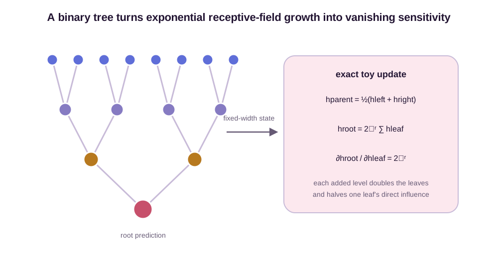
Alon and Yahav (2021) used this bottleneck view to explain why message-passing networks struggle on tasks that require matching information across distant tree leaves (Alon & Yahav, 2021). The argument extends beyond mean aggregation. A distant input affects a node through products of layer Jacobians along graph walks. When the number of relevant inputs grows faster than path capacity, or when normalized aggregation repeatedly attenuates each path, the Jacobian from a distant source to the target becomes small.

Increasing depth does not repair this attenuation merely by creating more walks. Di Giovanni et al. (2023) analyze width, depth, and topology in a common sensitivity framework. Their results show that width can mitigate over-squashing at the cost of greater overall sensitivity, while extra depth eventually faces vanishing-gradient effects. The largest obstruction comes from graph topology, especially node pairs with high commute time (Di Giovanni et al., 2023).

Commute time is the expected number of random-walk steps needed to travel from node \(u\) to node \(v\) and return. It is proportional to effective resistance, the electrical resistance obtained by treating every graph edge as a unit resistor:

\[\operatorname{Res}(u,v) = \frac{\tau(u,v)}{2\lvert E\rvert}.\]

Here, \(\tau(u,v)\) is commute time and \(\lvert E\rvert\) is the number of edges. Two nodes can have modest shortest-path distance but high effective resistance if all routes between them share a narrow cut. Effective resistance therefore detects global bottlenecks that hop count alone misses.

The commute-time identity is exact for an undirected connected graph with unit edge conductances (Chandra et al., 1989). It also gives a controlled scale check. On the five-node path \(P_5\), the two endpoints are connected by four unit resistors in series, so

\[\operatorname{Res}_{P_5}(v_0,v_4)=4.\]

The path has four edges, hence the endpoint commute time is \(2\cdot4\cdot4=32\) random-walk steps. Shortest-path distance and resistance happen to agree on a tree because every pair has a unique route. In a graph with parallel routes, resistance becomes smaller than distance and reveals the added capacity.

Curvature localizes topological bottlenecks

A dumbbell graph—two dense communities connected by one bridge—shows why topology dominates. Many signals from the left community must cross one edge to influence the right community. The bridge is not long, but it has low path redundancy. Deleting it disconnects the graph.

Discrete curvature gives a local language for this geometry. In a positively curved region, nearby nodes have overlapping neighborhoods and many short alternative routes. Across a negatively curved edge, the neighborhoods expand away from each other with few shared triangles or four-cycles. Topping et al. (2022) introduce an edge-based combinatorial curvature and connect highly negative curvature to sensitivity bottlenecks in message passing (Topping et al., 2022).

Curvature is a diagnostic, not a synonym for over-squashing. Over-squashing is defined by task-relevant sensitivity. Curvature describes topology without knowing the target. A negatively curved bridge is harmful when distant information must cross it; the same bridge is a useful locality prior when the task should ignore the other community.

The distinction can be made operational. Hold the dumbbell topology fixed and change only the label. If a node on the left must predict a bit stored on the right, sensitivity across the bridge is required, and the bridge curvature flags a plausible obstruction. If each node instead predicts its own community from local features, suppressing cross-bridge influence may improve the inductive bias. Curvature assigns the bridge the same score in both tasks. The task Jacobian

\[J_{uv} = \frac{\partial \widehat{y}_v}{\partial \mathbf{x}_u}\]

does not: it asks whether source \(u\) actually affects prediction \(v\) under the learned parameters and readout. Curvature is a topology-only proxy for where sensitivity may be difficult to transmit, while \(J_{uv}\) measures the model and task together.

No single proxy is decisive. High resistance with healthy distant Jacobians falsifies the claim that the observed failure is caused by squashing at that pair. Negative curvature with a purely local target is irrelevant. Conversely, a tiny distant Jacobian on a graph with low resistance points toward learned contraction, saturated nonlinearities, or optimization rather than a structural cut.

Rewiring trades locality for communication

If topology creates the bottleneck, one response is to separate the input graph from the computational graph. The input graph records observed relations. The computational graph records which nodes exchange messages. Adding edges across a narrow cut creates alternative routes and lowers effective resistance.

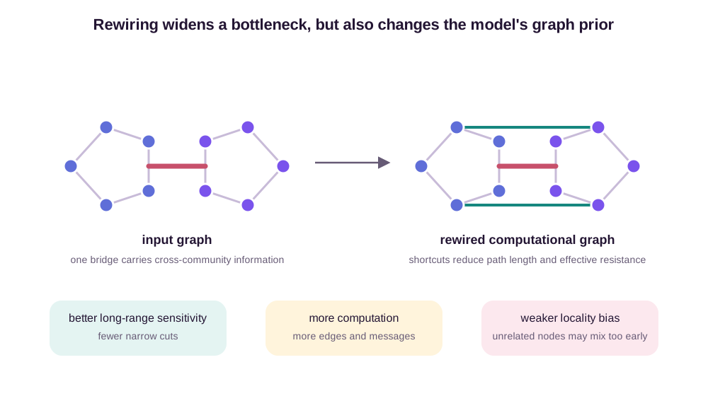
Rewiring is not free. A denser graph increases time and memory per layer. It makes unrelated nodes interact earlier and may erase the meaning of graph distance. It can also worsen over-smoothing because diffusion now has more routes. Full self-attention takes the limiting approach of connecting every node pair, reducing graph distance to one but typically paying quadratic cost and requiring positional or structural encodings to recover the original graph.

One shortcut improves transport and accelerates mixing

Return to the endpoints of \(P_5\). Add one edge \((v_0,v_4)\). The graph becomes the cycle \(C_5\). The new direct unit resistor lies in parallel with the original four-edge route, so the endpoint resistance is

\[\operatorname{Res}_{C_5}(v_0,v_4) = \left(1^{-1}+4^{-1}\right)^{-1} =0.8.\]

The graph now has five edges, giving commute time \(2\cdot5\cdot0.8=8\). A single shortcut reduces shortest-path distance from four to one, effective resistance from \(4\) to \(0.8\), and commute time from \(32\) to \(8\). For the endpoint-copy task from the opening section, the computational dependency becomes available after one layer instead of four on this smaller path.

The same edge also speeds diffusion. To compare mixing on these two graphs, use the lazy random-walk operator \(\mathbf{S}_{\mathrm{lazy}}=(\mathbf{I}+\mathbf{D}^{-1}\mathbf{A})/2\). For \(P_5\), its second-largest eigenvalue is

\[\lambda_2(P_5) = \frac{1+\cos(\pi/4)}{2} \approx0.8536.\]

For \(C_5\), it is

\[\lambda_2(C_5) = \frac{1+\cos(2\pi/5)}{2} \approx0.6545.\]

After ten linear propagation steps, the slowest non-stationary mode is scaled by about \(0.8536^{10}\approx0.205\) on the path but only \(0.6545^{10}\approx0.0144\) on the rewired cycle. The shortcut improves long-range transport and makes global mixing roughly fourteen times more aggressive at this depth. This is the central rewiring counterfactual: lower resistance can relieve over-squashing while worsening over-smoothing.

The calculation is exact for these lazy random walks. Treating the eigenvalue ratios as a prediction of a trained nonlinear GNN would again be an approximation. Their value is causal isolation: the features, task, and propagation rule are held fixed while one edge changes both the resistance and the mixing spectrum.

Dynamic rewiring tries to retain distance as an inductive bias. DRew adds connections as layers progress, so nodes at distance \(r\) begin communicating only when the network reaches the corresponding scale. Its delay mechanism can also use a less-smoothed state from the time when the source information first became available. Gutteridge et al. (2023) report that this progressive construction improves several long-range benchmarks without making every distant pair interact from the first layer (Gutteridge et al., 2023).

Hierarchical pooling offers another route. A coarsened graph can turn a long path into a short path between supernodes, much as image pyramids communicate over large spatial scales. The tradeoff moves into the pooling rule: an early merge can discard which fine-scale node contributed the signal. Global graph states provide a cheap communication hub, but compress the entire graph through one shared vector—the same bottleneck in a different location.

Molecular graphs make the choice concrete. A bond graph is a good computational prior for short-range covalent interactions. It is a poor communication graph for two atoms that are distant in bond count but close in three-dimensional space. Radius graphs, long-range electrostatic modules, or global attention can add the missing physical routes. Connecting every atom to every other atom may be unnecessary when the target is predominantly local. The right computational graph follows the interactions that matter, not graph density as an end in itself.

Diagnose the failure before choosing the remedy

Depth alone does not identify why a graph network fails. A useful diagnosis changes one mechanism at a time and asks for a falsifying outcome. The following matrix summarizes the controlled comparisons developed above.

Observable	Candidate mechanism	Matched intervention	Outcome that weakens the diagnosis
Prediction is invariant to a source feature until depth reaches the exact graph distance	Under-reaching	Add layers, a physically justified shortcut, or a global communication route	The shallow output already changes with that source, or added reach does not expose any new dependency
Dirichlet energy, pairwise distance, or class separation collapses with depth while distant Jacobians remain usable	Over-smoothing	Residual filtering, initial-feature injection, Jumping Knowledge, or controlled normalization	Feature contrast is restored but accuracy does not change; the lost frequency was not task-relevant
Distant task Jacobians decay with fan-in or path length; relevant pairs also have high resistance or cross a narrow cut	Over-squashing	Targeted rewiring, hierarchical routes, wider channels, or a global module	Rewiring lowers resistance but neither the distant Jacobian nor task performance changes under matched training
Training loss degrades with depth although linear propagation retains contrast and distant sensitivity	Optimization or parameterization	Identity-biased transformations, normalization, learning-rate or initialization changes	The same failure appears in a parameter-free propagation calculation
Two inputs receive the same representation for every parameter choice even at sufficient depth	Architectural expressivity ceiling	Change aggregation, identifiers, positional information, or higher-order state	Better optimization separates the pair under the unchanged architecture; then the collision was empirical rather than structural

The final row belongs to the expressivity chapter linked in the opening note, but it belongs in the differential diagnosis. An expressivity collision, under-reaching, smoothing, and squashing can all produce the same validation accuracy. Their quantifiers differ. Under-reaching says no local architecture of insufficient depth can depend on the distant input. An expressivity ceiling says no parameter choice in the stated architecture can separate a witness pair. Over-smoothing and over-squashing describe depth-dependent dynamics and sensitivity, so learned weights can mitigate or exacerbate them.

A practical intervention sequence

Start with the cheapest counterfactual. Mask or perturb a source feature and measure when the target output changes across depth. If influence appears only at the graph distance, communication range is binding. If influence appears and then node contrast collapses, compare vanilla, residual, and initial-injection propagation while holding width and training budget fixed. If contrast survives but distant influence stays tiny, measure Jacobians by distance and compare them with resistance or cut statistics.

Only then change topology. Add a small set of task-plausible shortcuts and record two curves: distant sensitivity and a smoothing statistic. A useful rewiring should improve the first without unacceptable damage to the second. Reporting only accuracy hides whether the shortcut repaired transport or merely changed regularization. Reporting only resistance hides whether the model learned to use the new edge.

Width is also a controlled intervention, not a universal cure. If doubling width increases distant Jacobian rank or task accuracy while the smoothing curve remains nearly fixed, channel capacity was binding. If the Jacobian remains exponentially small with distance, the extra coordinates did not repair the route. Global attention is the extreme topology intervention: it removes hop distance but can replace a sparse bottleneck with a computational and statistical one.

The central tension is unavoidable. Local message passing is efficient because it ignores most node pairs. Long-range tasks ask the model to recover some of those ignored interactions. A successful deep graph network does not remove locality indiscriminately. It decides which information should travel far, how quickly it should travel, and how much detail must survive the trip.

References

• Xu, K., Li, C., Tian, Y., Sonobe, T., Kawarabayashi, K., & Jegelka, S. (2018). Representation Learning on Graphs with Jumping Knowledge Networks. Proceedings of ICML. ↩
• Oono, K., & Suzuki, T. (2020). Graph Neural Networks Exponentially Lose Expressive Power for Node Classification. ICLR. ↩
• Chen, M., Wei, Z., Huang, Z., Ding, B., & Li, Y. (2020). Simple and Deep Graph Convolutional Networks. Proceedings of ICML. ↩
• Zhao, L., & Akoglu, L. (2020). PairNorm: Tackling Oversmoothing in GNNs. ICLR. ↩
• Alon, U., & Yahav, E. (2021). On the Bottleneck of Graph Neural Networks and its Practical Implications. ICLR. ↩
• Topping, J., Di Giovanni, F., Chamberlain, B. P., Dong, X., & Bronstein, M. M. (2022). Understanding Over-Squashing and Bottlenecks on Graphs via Curvature. ICLR. ↩
• Di Giovanni, F., Giusti, L., Barbero, F., Luise, G., Liò, P., & Bronstein, M. M. (2023). On Over-Squashing in Message Passing Neural Networks: The Impact of Width, Depth, and Topology. Proceedings of ICML. ↩
• Gutteridge, B., Dong, X., Bronstein, M. M., & Di Giovanni, F. (2023). DRew: Dynamically Rewired Message Passing with Delay. Proceedings of ICML. ↩
• Chandra, A. K., Raghavan, P., Ruzzo, W. L., Smolensky, R., & Tiwari, P. (1989). The Electrical Resistance of a Graph Captures Its Commute and Cover Times. Proceedings of STOC. ↩