On this page
Adapted from my 2025 Machine Learning for Molecules and Geometric Deep Learning lectures. The article follows a materials claim from composition and periodic structure through stability, properties, synthesis, and experimental closure.
A formula is not a material
Materials discovery is often drawn as an inverse problem: specify a desired property, then search for a chemical formula that provides it. That picture omits the variable that usually decides the answer. A material is a composition arranged into a structure, produced under conditions that may or may not realize that structure.
Consider a crystal with \(N\) atoms in one unit cell. Let \(\mathbf{L}=[\boldsymbol{\ell}_1,\boldsymbol{\ell}_2,\boldsymbol{\ell}_3]\in\mathbb{R}^{3\times 3}\) denote the lattice matrix, let \(\mathbf{s}_i\in[0,1)^3\) denote the fractional coordinate of atom \(i\), and let \(z_i\) denote its chemical element. Its Cartesian coordinate is
\[\mathbf{r}_i=\mathbf{L}\mathbf{s}_i.\]The finite tuple \(X=(\mathbf{L},\{(\mathbf{s}_i,z_i)\}_{i=1}^{N})\) represents the infinite periodic set
\[\mathcal{C}(X)=\left\{\left(\mathbf{L}(\mathbf{s}_i+\mathbf{n}),z_i\right): i=1,\ldots,N,\;\mathbf{n}\in\mathbb{Z}^3\right\}.\]The same infinite crystal admits many finite descriptions. We can permute atoms, translate the origin, wrap a fractional coordinate across a cell boundary, or choose another valid unit cell. A property model must give the same scalar prediction for all equivalent descriptions. When it predicts a vector or tensor, such as force or stress, its output must transform consistently with rotations and changes of basis.
Composition discards most of this information. Two crystals can share a reduced formula but differ in lattice, atomic coordination, or space group. Such polymorphs can have different band gaps, elastic constants, magnetic order, and kinetic accessibility. Figure 1 uses a generic A\(_2\)B\(_2\) composition to make the missing variable visible; the separate AB\(_3\) running candidate begins below.
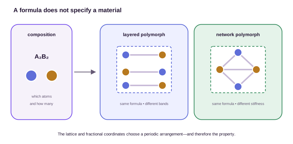
Crystal symmetry compresses this description further, but it does not remove structure. A space group collects the rotations, reflections, inversions, screw operations, glide operations, and translations that leave the crystal unchanged. Wyckoff positions group sites that are equivalent under these operations. Symmetry therefore constrains which coordinates are independent and which tensor components can be nonzero. It does not imply that two structures with the same composition—or even the same space group—have the same energy.
One crystal, several periodic files
The equivalence of periodic descriptions is easiest to see by constructing a supercell. Suppose a primitive cell of a hypothetical \(\alpha\)-AB\(_3\) phase contains one A atom and three B atoms. Replacing its lattice by
\[\mathbf{L}'=\mathbf{L} \begin{bmatrix} 2&0&0\\ 0&1&0\\ 0&0&1 \end{bmatrix}\]doubles the cell along the first lattice vector. The determinant of the integer matrix is \(2\), so the new cell has twice the volume and must contain two translated copies of every site: two A atoms and six B atoms. One copy keeps fractional coordinate \(\mathbf{s}_i'=(s_{i1}/2,s_{i2},s_{i3})\); the other uses \(\mathbf{s}_i'=((s_{i1}+1)/2,s_{i2},s_{i3})\). Both files generate exactly the same infinite set \(\mathcal{C}(X)\).
An intensive prediction such as band gap or density must be identical for the four-atom and eight-atom descriptions. An extensive prediction such as total cell energy must double. Per-atom energy must remain fixed. These are exact representation identities, not approximate augmentation rules. They provide simple tests for a crystal model: duplicate the cell and check whether its output scales with the physical quantity rather than with the file size.
The running candidate in this post is the hypothetical \(\alpha\)-AB\(_3\) polymorph. A second polymorph, \(\beta\)-AB\(_3\), has the same reduced formula but a different coordination network. We will ask whether \(\alpha\)-AB\(_3\) has the desired electronic and mechanical response, survives competition with other A–B phases, remains useful when defects and temperature are restored, and can be produced and identified experimentally.
The target is a property of a state
Materials are judged by different observables because applications ask different physical questions. For an electronic material, one common target is the band gap
\[E_{\mathrm{g}}=\min_{\mathbf{k}}E_{\mathrm{c}}(\mathbf{k})-\max_{\mathbf{k}}E_{\mathrm{v}}(\mathbf{k}),\]where \(E_{\mathrm{c}}(\mathbf{k})\) and \(E_{\mathrm{v}}(\mathbf{k})\) are the lowest conduction-band and highest valence-band energies at wavevector \(\mathbf{k}\). The minimizing and maximizing wavevectors need not agree, so the definition includes indirect gaps. The value also depends on the electronic-structure approximation: a density-functional-theory band gap is a calculated label, not an error-free experimental truth.
Mechanical response asks a different question. For a small strain tensor \(\boldsymbol{\varepsilon}\), the energy density can be expanded as
\[\frac{E(\boldsymbol{\varepsilon})}{V}=\frac{E(\mathbf{0})}{V}+\frac{1}{2}\sum_{i,j,k,l}C_{ijkl}\varepsilon_{ij}\varepsilon_{kl}+\mathcal{O}(\lVert\boldsymbol{\varepsilon}\rVert^3),\]where \(V\) is the cell volume and \(C_{ijkl}\) is the elastic tensor. Bulk and shear moduli are reductions of this tensor under specified averaging assumptions. A high bulk modulus does not imply fracture toughness, just as a useful band gap does not imply high carrier mobility.
Thermodynamic targets require another layer. For a phase at temperature \(T\) and pressure \(P\), the relevant potential is the Gibbs free energy
\[G(T,P)=E+PV-TS,\]where \(E\) is internal energy, \(V\) is volume, and \(S\) is entropy. High-throughput databases usually approximate solid-phase comparisons with relaxed electronic energies at zero temperature and low pressure. That approximation is useful because it is standardized and scalable. It cannot settle phase competition driven by vibrational, configurational, magnetic, or electronic entropy.
The choice of target must therefore name both the observable and the state. “Find a good conductor” is incomplete without temperature, carrier concentration, microstructure, and transport direction. “Find a stable crystal” is incomplete without competing phases, chemical environment, and thermodynamic conditions.
The AB3 target changes with the state definition
Assume the design brief asks for a room-temperature semiconductor with an electronic gap between \(1.6\) and \(2.0\) eV and a bulk modulus above \(120\) GPa. A standardized semilocal DFT calculation on relaxed, defect-free \(\alpha\)-AB\(_3\) gives \(E_{\mathrm{g}}^{\mathrm{PBE}}=1.35\) eV. That number is a state-specific surrogate label: zero-temperature geometry, one magnetic configuration, no defects, and a particular exchange–correlation approximation.
Suppose a more expensive quasiparticle calculation adds a \(0.45\) eV correction, while electron–phonon and thermal-expansion effects lower the gap by \(0.25\) eV at \(300\) K. Under the approximation that these corrections can be added,
\[E_{\mathrm{g}}(300\,\mathrm{K}) \approx1.35+0.45-0.25 =1.55\;\mathrm{eV}.\]The candidate changes from a pass at the high-fidelity electronic level, \(1.80\) eV, to a near miss under the stated operating condition. The additive correction is not an identity: lattice expansion can change the electronic correction, and disorder can make a single band edge ill-defined. Its purpose is to expose which omitted term changes the decision.
Mechanical screening needs the same precision. For a cubic approximation, the independent elastic constants are \(C_{11}\), \(C_{12}\), and \(C_{44}\). The Voigt bulk modulus is
\[K=\frac{C_{11}+2C_{12}}{3}.\]If strained calculations give \(C_{11}=210\) GPa, \(C_{12}=90\) GPa, and \(C_{44}=65\) GPa, then \(K=130\) GPa. The candidate passes the bulk-modulus threshold. It also satisfies the cubic mechanical-stability conditions \(C_{11}-C_{12}>0\), \(C_{44}>0\), and \(C_{11}+2C_{12}>0\). These conditions concern infinitesimal strain of an ideal single crystal. They do not establish fracture toughness or strength in a porous polycrystalline pellet.
Stability is a comparison, not a score
Formation energy is the first useful comparison. Suppose a crystal contains \(n_a\) atoms of element \(a\), with \(N=\sum_a n_a\). Given elemental reference energies \(\mu_a\), its formation energy per atom is
\[\Delta E_{\mathrm{f}}(X)=\frac{E(X)-\sum_a n_a\mu_a}{N}.\]A negative value means that the compound is lower in energy than its separated elements under the chosen reference calculation. It does not mean that the compound is the lowest-energy combination available at its composition. Other compounds may decompose it more favorably.
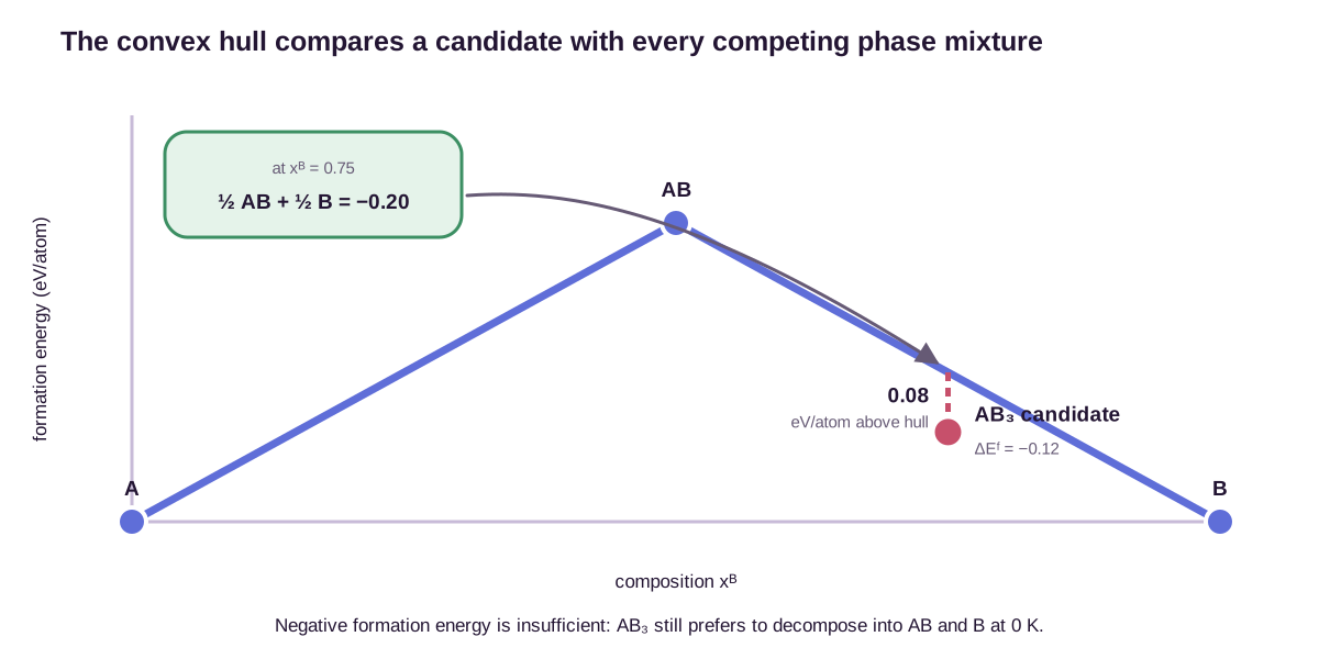
The convex hull supplies the missing comparison. Let \(\mathbf{x}^{(m)}\) and \(\Delta E_{\mathrm{f}}^{(m)}\) denote the composition vector and formation energy per atom of known or computed phase \(m\). At target composition \(\mathbf{x}\), the hull energy is
\[E_{\mathrm{hull}}(\mathbf{x})=\min_{\boldsymbol{\lambda}}\sum_m\lambda_m\Delta E_{\mathrm{f}}^{(m)}\]subject to
\[\lambda_m\geq 0,\qquad \sum_m\lambda_m=1,\qquad \sum_m\lambda_m\mathbf{x}^{(m)}=\mathbf{x}.\]The coefficients \(\lambda_m\) describe a phase mixture with the same overall composition. The energy above hull of candidate \(X\) is
\[\Delta E_{\mathrm{hull}}(X)=\Delta E_{\mathrm{f}}(X)-E_{\mathrm{hull}}(\mathbf{x}(X))\geq 0.\]For the binary example in Figure 2, the compound AB lies on the hull at \(-0.40\) eV per atom. A proposed AB₃ polymorph at composition \(x_{\mathrm{B}}=0.75\) has formation energy \(-0.12\) eV per atom. At the same composition, an equal mixture of AB and elemental B has energy \(-0.20\) eV per atom. The candidate is therefore \(0.08\) eV per atom above the hull even though its formation energy is negative.
A competing phase can reverse a screening decision
The first hull is provisional because it contains only AB and the elements. Suppose a later search finds AB\(_2\) at B fraction \(2/3\) with formation energy \(-0.30\) eV per atom. To reproduce the AB\(_3\) composition, mix a fraction \(\lambda\) of AB\(_2\) with \(1-\lambda\) elemental B:
\[\lambda\left(\frac{2}{3}\right)+(1-\lambda)(1)=\frac{3}{4}.\]Solving gives \(\lambda=3/4\). The competing mixture now has energy
\[E_{\mathrm{mix}} =\frac{3}{4}(-0.30)+\frac{1}{4}(0) =-0.225\;\mathrm{eV/atom}.\]The same \(\alpha\)-AB\(_3\) energy therefore lies \(-0.12-(-0.225)=0.105\) eV per atom above the expanded hull. A screening rule that retains candidates below \(0.10\) eV per atom would have accepted the old result and rejected the new one. Nothing about \(\alpha\)-AB\(_3\) changed; the comparison set did.
Uncertainty and temperature change the ranking again
Energy uncertainty matters through differences, not isolated error bars. Write the candidate and mixture energies as random variables \(E_c\) and \(E_m\). Their difference has variance
\[\operatorname{Var}(E_c-E_m) =\sigma_c^2+\sigma_m^2-2\rho\sigma_c\sigma_m,\]where \(\rho\) is their error correlation. Shared elemental references and systematic functional errors can make \(\rho\) positive, so adding independent error bars in quadrature may overstate uncertainty. Conversely, different bonding motifs can have weakly correlated biases.
For a simple independent-error estimate, take \(\sigma_c=0.040\) eV per atom and \(\sigma_{\mathrm{AB_2}}=0.020\) eV per atom. Elemental B defines the zero, so the uncertainty of the three-quarter AB\(_2\) mixture is \(0.75(0.020)=0.015\) eV per atom. The uncertainty in energy above hull is then
\[\sigma_{\mathrm{hull}} =\sqrt{0.040^2+0.015^2} \approx0.043\;\mathrm{eV/atom}.\]Thus the nominal \(0.105\) eV per atom result is only about \(2.4\) standard deviations above zero under these assumptions. An uncertainty-aware workflow should send the candidate to a more accurate calculation rather than turn the mean into a binary certificate.
Now restore a toy finite-temperature correction at a proposed synthesis temperature of \(900\) K. Assume vibrational and configurational terms lower the free energy of defect-tolerant \(\alpha\)-AB\(_3\) by \(0.080\) eV per atom, while they lower AB\(_2\) by only \(0.010\) eV per atom. Elemental B again defines zero for this illustration. The candidate and competing mixture become
\[G_c=-0.120-0.080=-0.200\;\mathrm{eV/atom},\] \[G_m=\frac{3}{4}(-0.300-0.010)=-0.2325\;\mathrm{eV/atom}.\]The finite-temperature distance to the hull is now \(0.0325\) eV per atom. The candidate moves from rejection at \(0\) K to retention under a \(0.05\) eV per atom finite-temperature threshold. The numerical corrections are hypothetical, and a real calculation would need phonons, configurational sampling, and consistent free energies for every competing phase. The decision change is the point: a temperature correction applied only to the candidate would be invalid because stability remains a comparison.
This construction underlies large computed resources such as the Materials Project (Jain et al., 2013). It also exposes three boundaries around any claim of stability.
First, a hull is only as complete as its phase set. A newly discovered lower-energy competitor can move an older candidate off the hull. Merchant et al. explicitly observed this effect when expanding the candidate set with large-scale graph-network screening (Merchant et al., 2023). Second, the energies share the systematic and numerical errors of the chosen electronic-structure workflow. Comparing energies computed with incompatible reference schemes can invalidate the hull. Third, the usual computed hull describes a closed system near zero temperature. Open chemical reservoirs, pressure, and entropy require a different thermodynamic potential or additional free-energy terms.
An energy above hull is thus a decomposition driving force within a declared model, not a universal synthesizability probability. Empirically observed metastability spans chemistry-dependent energy scales; polymorphs and phase-separating compounds show different distributions (Sun et al., 2016). Kinetic trapping can preserve an above-hull phase, while a predicted ground state can remain inaccessible because nucleation and diffusion are too slow.
The physical material exceeds the ideal cell
A relaxed, defect-free periodic cell is an intentionally narrow object. Real specimens may contain vacancies, interstitials, substitutions, dislocations, grain boundaries, surfaces, amorphous regions, and mixtures of polymorphs. Their concentrations depend on chemical potentials and processing history.
For a neutral defect, a simplified formation energy is
\[E_{\mathrm{def}}^{\mathrm{f}}=E_{\mathrm{def}}-E_{\mathrm{bulk}}-\sum_a\Delta n_a\mu_a,\]where \(E_{\mathrm{def}}\) and \(E_{\mathrm{bulk}}\) are matched supercell energies and \(\Delta n_a\) counts atoms added to the defective cell. Charged defects add Fermi-level and electrostatic finite-size terms. Even the neutral expression shows why a defect concentration is not an intrinsic number attached to a formula: it varies with the allowed chemical reservoirs \(\mu_a\).
Defect thermodynamics turns reservoirs into concentrations
In the dilute, non-interacting approximation, the equilibrium fraction of available sites occupied by a defect is
\[c\approx g\exp\!\left(-\frac{\Delta G_{\mathrm{def}}^{\mathrm{f}}}{k_{B}T}\right),\]where \(g\) is a degeneracy factor and \(\Delta G_{\mathrm{def}}^{\mathrm{f}}\) is the defect formation free energy. This relation follows by balancing the energetic penalty against the configurational entropy of distributing a small number of defects over many sites. It breaks down when defects interact, cluster, or reach concentrations large enough to alter the host phase.
For \(\alpha\)-AB\(_3\), consider a B vacancy with \(g=1\). At \(900\) K, \(k_{B}T\approx0.0776\) eV. Under B-rich conditions, suppose \(\Delta G_{V_{\mathrm{B}}}^{\mathrm{f}}=0.70\) eV. The predicted fraction of vacant B sites is
\[c_{\mathrm{B-rich}} \approx e^{-0.70/0.0776} \approx1.2\times10^{-4}.\]Under B-poor conditions, the chemical-potential term lowers the formation free energy to \(0.35\) eV, giving
\[c_{\mathrm{B-poor}} \approx e^{-0.35/0.0776} \approx1.1\times10^{-2}.\]Changing the reservoir produces roughly a hundredfold concentration change without altering the ideal crystal file. The exponent makes a formation-energy error of \(0.10\) eV a concentration factor of \(e^{0.10/0.0776}\approx3.6\) at the same temperature. Defect predictions therefore require tighter energy consistency than a coarse screening rank. The standard first-principles defect formalism makes the chemical-potential, charge-state, and finite-size terms explicit (Van de Walle and Neugebauer, 2004).
The vacancy can also change the target property. Assume each ionized B vacancy contributes one mobile electron, the B-site density is \(3\times10^{22}\) cm\(^{-3}\), and the electron mobility is \(2\) cm\(^2\) V\(^{-1}\) s\(^{-1}\). The conductivity estimate \(\sigma=nq\mu\) gives about \(1.2\) S/cm in the B-rich case and \(106\) S/cm in the B-poor case. These numbers use complete ionization and constant mobility, both strong assumptions. They show why a defect-free band gap and a measured conductivity answer different questions.
At finite temperature, a more useful solid free-energy approximation may include vibrational and configurational contributions,
\[G(T,P)\approx E_{\mathrm{DFT}}+F_{\mathrm{vib}}(T)-TS_{\mathrm{config}}+PV.\]These terms can reorder polymorphs that are close in electronic energy. Thermal expansion can change a band structure. A small dopant concentration can dominate conductivity. Grain size can change strength. Figure 3 summarizes why a bulk-cell prediction and a measured material property are different claims.
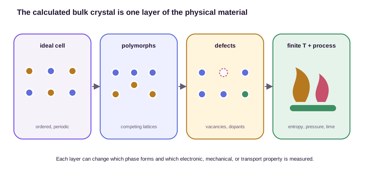
The distinction prevents two common overclaims. Predicting a low energy for one ordered structure does not establish that the material forms as a pure phase. Predicting a property for that structure does not establish that a processed sample retains the same property.
Property prediction must respect periodic structure
A structure-aware predictor learns a map \(f_{\theta}:X\mapsto y\) from a periodic crystal \(X\) to a property \(y\). Crystal graph neural networks represent atoms as nodes and connect each atom to neighbors, including periodic images. Xie and Grossman showed that message passing over such local environments can learn crystal properties from structure (Xie and Grossman, 2018). Modern variants add angular information, equivariant tensor features, or learned interatomic potentials.
Periodic edges belong to the infinite crystal
For atoms \(i\) and \(j\) in the stored cell, a periodic neighbor is indexed not only by the pair \((i,j)\) but also by a lattice shift \(\mathbf{n}\in\mathbb{Z}^3\). Its displacement is
\[\mathbf{d}_{ij\mathbf{n}} =\mathbf{L}(\mathbf{s}_j-\mathbf{s}_i+\mathbf{n}).\]An edge enters a cutoff graph when \(\lVert\mathbf{d}_{ij\mathbf{n}}\rVert<r_{\mathrm{cut}}\). This definition automatically connects an atom near one cell face to a neighbor stored near the opposite face. Building edges only from Cartesian coordinates inside the displayed cell would treat the artificial boundary as a surface.
The four-atom and doubled eight-atom descriptions of \(\alpha\)-AB\(_3\) should produce the same multiset of local environments per atom. If the network predicts an intensive property, mean pooling preserves the answer. If it predicts total energy through atomic contributions,
\[E_{\theta}(X)=\sum_{i=1}^{N}\varepsilon_{\theta}(\mathcal{N}_i),\]then duplicating the cell duplicates the sum. Here \(\mathcal{N}_i\) is atom \(i\)’s periodic neighborhood and \(\varepsilon_{\theta}\) is a learned local energy surrogate. This construction gives the required extensivity, but locality is still an approximation. Long-range electrostatics, collective strain, and delocalized electronic states can exceed the cutoff.
The representation must preserve the equivalences of the crystal. For a scalar property,
\[f_{\theta}(X)=f_{\theta}(g\cdot X)\]for every transformation \(g\) that changes the description but not the physical crystal. These transformations include atom permutations, periodic translations, rigid rotations, and valid cell reparameterizations. A model that is invariant to atom order but sensitive to which equivalent unit cell happens to be stored in a file has learned a data convention, not a material property.
Fast predictors enable large screening funnels, but test error alone does not validate a discovery claim. Random train-test splits can place near-duplicate structures or related polymorphs on both sides. A model trained near relaxed minima may fail on the distorted structures encountered during relaxation. A band-gap model inherits the bias of its computational labels. Evaluation should therefore separate chemical systems, structural prototypes, or time periods according to the intended deployment.
Uncertainty is equally conditional. An ensemble disagreement score can flag inputs far from training data, but low disagreement does not reveal a bias shared by every model. Uncertainty should decide which candidate receives a more accurate calculation or experiment; it should not be treated as a certificate of correctness.
For the running candidate, suppose five models predict the semilocal gap as \(1.42\pm0.05\) eV. The small spread does not cover the difference between that label and the corrected room-temperature target developed earlier. Every ensemble member learned the same semilocal training labels, so all can agree on the same biased quantity. A useful evaluation would hold out the AB\(_3\) structural prototype, test both primitive and supercell descriptions, and compare the final corrected quantity against the deployment threshold. A random split over database rows tests interpolation among stored conventions instead.
Inverse design generates hypotheses
Forward prediction asks for \(p(y\mid X)\): what property follows from this crystal? Inverse design seeks structures consistent with a target, which can be written schematically as
\[p(X\mid y^{\star})\propto p(y^{\star}\mid X)p(X).\]The prior \(p(X)\) matters. It encodes which compositions, lattices, symmetries, and local environments the generator regards as plausible. A conditional generator can sample element types, lattice parameters, and fractional coordinates, then steer samples toward a target property. MatterGen, for example, jointly denoises atom types, coordinates, and lattices and conditions generation on chemical, symmetry, and scalar-property constraints (Zeni et al., 2025).
The raw sample is the beginning of a screening funnel. A defensible workflow checks charge and composition constraints, relaxes the structure, removes duplicates, recomputes properties at higher fidelity, and rebuilds the convex hull with relevant competing phases. Many generated crystals move substantially during relaxation or collapse to the same minimum. Novelty before relaxation is not novelty after relaxation.
Multi-objective design makes the funnel narrower. A battery electrolyte may need ionic conductivity, electrochemical stability, mechanical compatibility, low electronic conductivity, available elements, and a viable processing window. These conditions rarely reduce to a single weighted score without value judgments. Pareto fronts keep the tradeoffs visible: a candidate is Pareto optimal when no other candidate improves one objective without worsening another.
Joint feasibility is narrower than three good means
Apply the same logic to \(\alpha\)-AB\(_3\) at the cheaper inverse-design stage, before the explicit correction stack used in the Target Is a Property of a State section. After relaxation, assume calibrated surrogates predict a room-temperature gap of \(1.78\pm0.10\) eV, energy above the finite-temperature hull of \(0.035\pm0.025\) eV per atom, and bulk modulus of \(128\pm8\) GPa. The constraints are
\[1.6<E_{\mathrm{g}}<2.0\;\mathrm{eV}, \qquad \Delta G_{\mathrm{hull}}<0.05\;\mathrm{eV/atom}, \qquad K>120\;\mathrm{GPa}.\]Approximating each prediction as Gaussian gives feasibility probabilities of about \(0.95\), \(0.73\), and \(0.84\). If their errors were independent, the probability of satisfying all three would be their product, about \(0.58\). Correlation can raise or lower that value; for example, volume errors may affect both gap and modulus. The independence calculation is therefore an approximation, but it reveals why three passing means do not imply a high-confidence candidate.
The later state-specific calculation moved the gap estimate from the surrogate mean of \(1.78\) eV to \(1.55\) eV and changed that constraint from pass to fail. Calibration describes frequencies over a population; it does not guarantee that one candidate lies inside its reported interval. This is why inverse design produces candidates for a fidelity ladder rather than final answers.
This probability changes the design decision. A generator that produces \(10{,}000\) nominal samples may yield \(1{,}200\) unique relaxed structures, \(180\) with passing mean predictions, and only about \(104\) expected to satisfy the three constraints under calibrated uncertainty. Element availability, charge balance, and synthesis constraints reduce the set further. Reporting \(180/10{,}000\) as the success rate mixes generation failures, duplicate collapse, and property uncertainty; each denominator answers a different question.
The output of inverse design is therefore a ranked hypothesis with a computational audit trail. Calling a generated file a discovered material skips relaxation, phase competition, synthesis, and measurement.
Synthesizability belongs to a process
Synthesis is better represented as a conditional outcome than as a label on the final structure. Let \(\mathbf{c}\) describe precursors, stoichiometry, temperature schedule, pressure, atmosphere, mixing, and time. Then a synthesis model asks for
\[p(\text{phase},\text{yield},\text{impurities}\mid X,\mathbf{c}),\]not merely whether \(X\) is “synthesizable.” The same target can form from one precursor set and fail from another because stable intermediates block the pathway. Increasing temperature can accelerate diffusion but stabilize a competing phase or volatilize a precursor. Pressure can change both equilibrium and kinetics.
Published recipes provide incomplete supervision for this problem. Successful conditions are reported more often than failed attempts, and small procedural details may be absent. Raccuglia et al. showed that archived unsuccessful reactions contain useful boundaries on crystallization conditions (Raccuglia et al., 2016). Negative results are not merely zeros in a table: the observed impurity phase can reveal which branch of the reaction network the experiment followed.
Autonomous laboratories make the conditional nature of synthesis operational. The A-Lab combined computed phase stability, literature-derived synthesis heuristics, robotic solid-state synthesis, X-ray diffraction, and active selection of follow-up recipes (Szymanski et al., 2023). It synthesized 36 of 57 proposed targets during its autonomous campaign. The failures included slow kinetics, precursor volatility, amorphization, and computational error—different causes that a single synthesizability score would merge.
A process window balances formation and loss
For the hypothetical candidate, consider the solid-state route
\[\mathrm{AB_2+B\longrightarrow \alpha\text{-}AB_3}.\]Too little thermal activation leaves AB\(_2\) unreacted; too much causes volatile B loss and returns the sample toward AB\(_2\). A toy kinetic model makes the tradeoff explicit. Let the target-formation and B-loss rates be
\[k_{\mathrm{form}}=10^7\exp\!\left(-\frac{1.8\;\mathrm{eV}}{k_{B}T}\right)\;\mathrm{s}^{-1},\] \[k_{\mathrm{loss}}=10^9\exp\!\left(-\frac{2.4\;\mathrm{eV}}{k_{B}T}\right)\;\mathrm{s}^{-1}.\]These prefactors and barriers are hypothetical effective parameters, not first-principles identities. At \(900\) K, they give a formation time \(1/k_{\mathrm{form}}\approx20\) minutes and a B-loss fraction \(1-e^{-k_{\mathrm{loss}}t}\approx6\%\) during a \(30\)-minute hold. At \(1000\) K, formation takes about two minutes, but the same hold loses roughly \(77\%\) of B. Heating faster is not automatically better.
The usable process window is the intersection of inequalities: formation must finish within the allowed hold, B loss must remain below tolerance, the container must survive, and the atmosphere must keep the desired chemical potentials. Increasing B partial pressure can suppress loss, while quenching can retain the finite-temperature phase after formation. A synthesis model should predict this window and its competing products, not attach one probability to the target structure.
Experimental closure changes the model
A discovery loop should choose the next experiment by both scientific value and information value. If candidate \(X\) has predicted utility \(u(X)\), uncertainty \(\sigma(X)\), and experimental cost \(c(X)\), a simple acquisition score is
\[a(X)=u(X)+\kappa\sigma(X)-\lambda c(X),\]where \(\kappa\) controls exploration and \(\lambda\) penalizes cost. In practice, diversity constraints prevent the batch from spending its entire budget on near-duplicates. Feasibility constraints prevent the acquisition function from repeatedly proposing unavailable precursors or incompatible apparatus.
Figure 4 shows the full loop. Computation proposes and ranks structures. Synthesis tests a route under recorded conditions. Characterization identifies phases, impurities, yield, microstructure, and the target property. The outcome then updates the property model, the synthesis model, the uncertainty estimate, or all three.
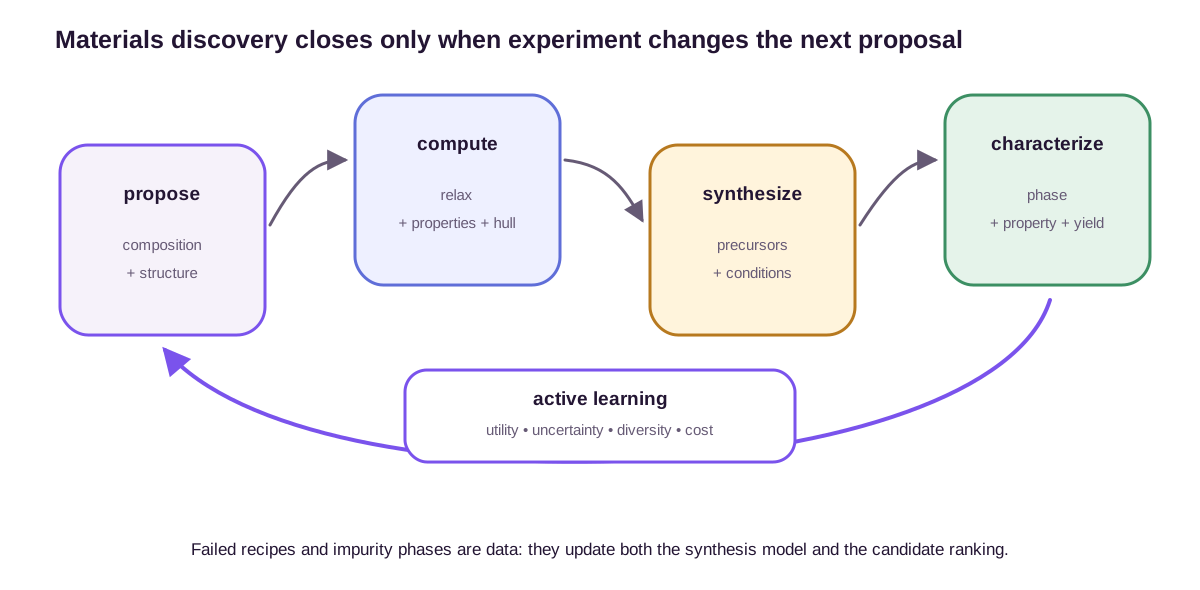
Experimental validation must match the original claim. Powder X-ray diffraction can test bulk phase identity and estimate phase fractions, but it may not resolve a small defect population. Microscopy can reveal local defects but samples a limited region. A measured conductivity needs specimen geometry, temperature, density, and contact protocol. Agreement on one observable does not validate the entire predicted structure-property chain.
Characterization must close the same claim that design opened
Suppose the first AB\(_3\) synthesis yields a powder diffraction refinement of \(82\%\) \(\alpha\)-AB\(_3\), \(15\%\) AB\(_2\), and \(3\%\) elemental B by mass. The diffraction result supports formation of the target phase but rejects the stronger claim of a phase-pure material. Rietveld refinement estimates phase fractions by fitting the full diffraction pattern rather than assigning isolated peaks (Rietveld, 1969); preferred orientation, amorphous content, and overlapping peaks remain model-dependent errors.
An optical absorption edge at \(1.62\) eV would fall inside the requested range, but it would not yet validate the predicted intrinsic gap of \(\alpha\)-AB\(_3\). The AB\(_2\) impurity, vacancy absorption, excitons, and the fitting convention can all shift the apparent onset. Phase-resolved spectroscopy or a purer specimen is needed. Likewise, nanoindentation measures a local indentation modulus, not the hydrostatic bulk modulus \(K=130\) GPa computed for a defect-free single crystal.
The failed purity claim still improves the loop. Residual AB\(_2\) suggests incomplete formation, whereas elemental B suggests that simply adding more B may overshoot locally. The next experiment could extend milling to shorten diffusion distances while keeping the \(900\) K hold, rather than raising temperature into the volatility regime. Its information value comes from distinguishing a kinetic bottleneck from an incorrect phase-stability calculation.
A complete prospective report keeps the denominators visible. Imagine starting with \(10{,}000\) generated files, obtaining \(1{,}200\) unique relaxed structures, selecting \(20\) for high-fidelity calculations, attempting \(6\) syntheses, forming the target phase in \(3\), and meeting phase-purity plus property criteria in \(1\). The end-to-end yield is \(1/10{,}000\), the experimental hit rate is \(3/6\) for target-phase formation, and the qualified-material rate is \(1/6\). None of these ratios replaces the others.
Prospective evaluation is the strongest test because the candidate and protocol are fixed before the outcome is known. Independent replication is stronger still. The proof-of-concept synthesis in MatterGen measured the target property of a generated material within 20% of the requested value, but the result validates one end-to-end case rather than a universal success rate. Claim boundaries should remain this narrow.
Materials discovery succeeds when a structure exists in more than a database. The composition must admit a periodic arrangement with the desired calculated response. That arrangement must compete favorably enough with other phases under relevant conditions. A process must form it, characterization must identify it, and measurement must confirm the property. Machine learning can accelerate every link, but no link substitutes for the next one.
References
Jain, A., Ong, S. P., Hautier, G., et al. (2013). The Materials Project: A materials genome approach to accelerating materials innovation. APL Materials, 1, 011002. ↩
Xie, T. & Grossman, J. C. (2018). Crystal graph convolutional neural networks for an accurate and interpretable prediction of material properties. Physical Review Letters, 120, 145301. ↩
Sun, W., Dacek, S. T., Ong, S. P., et al. (2016). The thermodynamic scale of inorganic crystalline metastability. Science Advances, 2, e1600225. ↩
Raccuglia, P., Elbert, K. C., Adler, P. D. F., et al. (2016). Machine-learning-assisted materials discovery using failed experiments. Nature, 533, 73–76. ↩
Merchant, A., Batzner, S., Schoenholz, S. S., et al. (2023). Scaling deep learning for materials discovery. Nature, 624, 80–85. ↩
Szymanski, N. J., Rendy, B., Fei, Y., et al. (2023). An autonomous laboratory for the accelerated synthesis of inorganic materials. Nature, 624, 86–91. ↩
Zeni, C., Pinsler, R., Zügner, D., et al. (2025). A generative model for inorganic materials design. Nature, 639, 624–632. ↩
Van de Walle, C. G. & Neugebauer, J. (2004). First-principles calculations for defects and impurities: Applications to III-nitrides. Journal of Applied Physics, 95, 3851–3879. ↩
Rietveld, H. M. (1969). A profile refinement method for nuclear and magnetic structures. Journal of Applied Crystallography, 2, 65–71. ↩