On this page
Adapted from my 2025 Machine Learning for Molecules and Geometric Deep Learning lectures. This article asks which sequence, backbone, motif, and joint distributions protein models generate—and what evidence survives the full design funnel. For the biological workflow and current tool landscape, begin with Protein Design.
Protein Design Is Not Structure Prediction in Reverse
A structure predictor starts with a sequence and asks which three-dimensional arrangement is compatible with it. Protein design begins with a much less complete specification: bind this target, hold these catalytic residues in place, assemble with a chosen symmetry, or merely create a stable fold unlike known ones. There is usually no unique sequence and often no unique backbone that satisfies such a request. The task is therefore not to invert a deterministic map. It is to sample from a large set of molecular solutions while retaining the constraints that matter.
Let \(a=(a_1,\ldots,a_L)\) denote an amino-acid sequence, \(X\) a backbone or all-atom structure, and \(y\) a desired property or function. Several distributions commonly called “protein design” are actually different problems:
\[\begin{aligned} \text{sequence generation:} &\qquad p_\theta(a\mid y),\\ \text{inverse folding:} &\qquad p_\theta(a\mid X),\\ \text{backbone generation:} &\qquad p_\theta(X\mid y),\\ \text{co-design:} &\qquad p_\theta(a,X\mid y). \end{aligned}\]The distinction is operational. A sequence model conditioned on a family label must still establish that its sample folds. An inverse-folding model inherits a target backbone, but must find a sequence whose physical energy landscape actually favors that backbone. A backbone generator can satisfy an elegant geometric constraint while leaving unanswered whether any sequence realizes it. A co-design model couples the two variables, but coupling does not make function observable from training data.
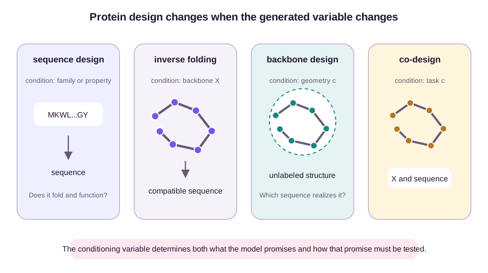
This viewpoint connects naturally to protein representation learning: sequence, residue graph, surface, and coordinate representations expose different constraints. It also clarifies why a highly capable structure predictor is valuable inside a design pipeline without itself becoming a design oracle. Prediction asks whether a proposed sequence is structurally plausible. Design asks how to search among proposals, and function is usually farther downstream than structure.
One hypothetical design will carry those distinctions. We want a 100-residue protein whose residues 18, 52, and 79 coordinate a zinc ion through a histidine–aspartate–histidine motif. The desired coordinating-atom distances are 2.1, 2.0, and 2.2 angstroms, and the three pairwise angles around the metal are 110, 108, and 109 degrees. The motif specifies local chemistry and geometry. It does not specify the remaining 97 residues, the global fold, the stability of that fold, solvent access, or measurable metal affinity.
A sequence generator can propose the three identities and their context. Inverse folding can populate a chosen scaffold. Backbone diffusion can construct the scaffold around fixed coordinating atoms. Co-design can revise sequence and geometry together. Each formulation transfers a different uncertainty to the next stage, so the same design will serve as a ledger rather than as nine unrelated examples.
Sequence Models Learn What Evolution Has Already Accepted
The largest source of protein data is sequence. An autoregressive model factors a distribution over amino acids as
\[p_\theta(a\mid y)=\prod_{i=1}^{L}p_\theta(a_i\mid a_{<i},y),\]while a masked or discrete-diffusion model repeatedly reconstructs corrupted residues. In both cases, conditioning \(y\) may encode a protein family, molecular function, organism, partial sequence, or textual annotation. ProGen demonstrated that a large conditional language model could generate sequences with controllable protein-family labels and that selected artificial lysozymes retained measurable activity despite substantial sequence divergence from natural proteins (Madani et al., 2023).
The strength of this formulation is also its limitation. Evolutionary sequence databases contain examples that survived folding, expression, cellular context, and historical selection. A language model compresses these regularities into a prior over plausible sequence space. But the database rarely contains controlled labels for a quantitative engineering objective such as “bind target \(T\) with nanomolar affinity while avoiding off-target \(T'\).” Annotation is incomplete, homologous families are unevenly sampled, and phylogeny produces many near-duplicates. A high model likelihood therefore means “resembles patterns accepted in the training distribution,” not “has the requested laboratory phenotype.”
One can formalize property guidance with Bayes’ rule:
\[p(a\mid y)\propto p(y\mid a)\,p(a).\]Here \(p(a)\) is a generative prior and \(p(y\mid a)\) is a fitness model, classifier, docking score, or another oracle. In log space, guided sampling often resembles optimizing
\[\log p(a)+\lambda\log p(y\mid a),\]where \(\lambda\) controls the pressure toward the requested property. Small \(\lambda\) leaves the prior dominant; large \(\lambda\) rewards whatever inputs exploit the oracle. The latter is a familiar failure of optimization under a learned surrogate: sequences can move far outside the oracle’s training support and receive extreme predicted scores for accidental reasons. The generator has not discovered biology merely because it has found the classifier’s blind spot.
This is especially consequential under epistasis. If the effect of mutating residue \(i\) depends on residue \(j\), a fitness surface cannot be reconstructed by adding single-mutation effects. A sequence generator can model such dependencies, but guidance based on a sparse assay may still be unreliable in novel combinations. Plausibility and task fitness are complementary signals, not interchangeable ones.
Additive guidance can reject an epistatic solution
Consider two context residues near the metal pocket. Encode the reference identities by \((z_1,z_2)=(0,0)\) and substitutions by 1. Suppose the measured fitness relative to the reference is
| \(z_1\) | \(z_2\) | True fitness change |
|---|---|---|
| 0 | 0 | 0 |
| 1 | 0 | -1 |
| 0 | 1 | -1 |
| 1 | 1 | +4 |
An additive guide estimated from the two single mutants predicts the double-mutant change as \(-1-1=-2\) and suppresses it. The true interaction term is
\[\epsilon_{12} =4-(-1)-(-1)-0 =6.\]The double substitution is favorable only as a pair—for example, one residue opens space while the other supplies the compensating hydrogen bond. Raising guidance strength \(\lambda\) makes this error worse because it concentrates sampling around the misspecified additive score. A joint sequence prior may assign the pair nonzero probability from evolutionary correlations, but multiplying it by a sufficiently sharp additive oracle can still remove the solution.
The remedy is not simply a larger generator. The property dataset must contain combinatorial interventions or a mechanistic representation that identifies the interaction. Prospective sampling should retain a control fraction from the unguided or weakly guided prior, otherwise the campaign cannot discover that the guide excluded the best epistatic region.
Inverse Folding Conditions on the Answer’s Geometry
Suppose a backbone \(X\) is fixed. The inverse-folding problem asks for sequences compatible with that geometry. An autoregressive version uses
\[p_\theta(a\mid X)=\prod_{i=1}^{L}p_\theta(a_{\pi_i}\mid a_{\pi_{<i}},X),\]where \(\pi\) is a decoding order. A geometric encoder passes messages between residues that are close in 3D, allowing a residue’s identity to depend on its spatial environment rather than only its neighbors along the chain. ProteinMPNN showed that this structure-conditioned formulation could design sequences with strong experimental recovery and folding behavior across monomers, oligomers, and protein–protein interfaces (Dauparas et al., 2022).
Consider a small helical bundle whose backbone is already specified. Residues buried in the core need mutually compatible size and hydrophobicity; exposed positions can often vary widely; a charged surface pair may be chosen to improve solubility without changing the fold. The backbone does not uniquely determine the sequence. It defines a conditional family of sequences, and sampling that family is useful precisely because multiple solutions can be screened for expression, stability, immunogenicity, or manufacturing constraints.
Yet inverse folding solves a compatibility problem, not the full thermodynamic problem. Training structures are typically single native conformations. The model learns which sequences occur on such backbones, but not necessarily the energy gap between the target and every competing fold, the rate of aggregation, or the effect of a cellular environment. Recovery of a native amino acid is also an imperfect metric: nature chose one residue under many historical constraints, whereas several alternatives may work. The more direct computational test is self-consistency—whether an independently predicted structure for the designed sequence returns to the target backbone. Even that test is evidence about structural agreement, not function.
Designability is a distribution, not one successful sequence
For a fixed backbone, conditional sequence entropy provides one limited view of designability:
\[H(A\mid X) =-\sum_a p(a\mid X)\log p(a\mid X).\]Its exponential, \(\exp H(A\mid X)\), is the effective number of comparably weighted sequences under the model. This is not a thermodynamic count, but it distinguishes a backbone supported by many sequence solutions from one balanced on a narrow model mode.
Freeze the zinc motif identities at positions 18, 52, and 79. Suppose two remaining core positions each admit leucine, isoleucine, or valine. For scaffold A, each position has probabilities \((0.5,0.3,0.2)\). Its per-position entropy is about 1.030 nats, so
\[H_A=2(1.030)=2.060, \qquad \exp(H_A)\approx7.84.\]For scaffold B, each position has probabilities \((0.9,0.05,0.05)\). Its per-position entropy is about 0.394 nats, giving
\[H_B=0.788, \qquad \exp(H_B)\approx2.20.\]Both scaffolds may yield one top sequence that refolds with low RMSD. Scaffold A nevertheless offers roughly 3.6 times more effective local sequence diversity for optimization or rescue mutations. High entropy alone is not automatically good: a diffuse conditional may reflect uncertainty or poor geometry rather than genuine physical tolerance. The useful comparison combines entropy with the fraction of independently sampled sequences that refold, remain monomeric, and preserve the motif.
Backbone Generation Searches a Geometric Space
Inverse folding becomes more powerful when the backbone itself need not be borrowed from nature. A backbone generator represents a protein as residue coordinates or local rigid frames and learns a distribution over fold-like geometries. In a simplified coordinate diffusion process,
\[X_t=\alpha_t X_0+\sigma_t\epsilon, \qquad \epsilon\sim\mathcal N(0,I),\]and a denoising network estimates either \(X_0\), the added noise, or the score \(\nabla_{X_t}\log p_t(X_t)\). Sampling starts from noise and integrates the learned reverse process toward a structured backbone. Real systems must respect more than this schematic equation: global translation and rotation should not change probability, local frames live on rotation groups, chain connectivity produces correlated rather than independent geometry, and chirality must be preserved. These are architectural constraints, not cosmetic data augmentation.
RFdiffusion adapted a structure-prediction network to denoising and generated monomers, symmetric assemblies, binders, and scaffolds around functional motifs, with experimental tests spanning structure and function (Watson et al., 2023). Chroma likewise combined structured diffusion with sequence and side-chain design and showed conditional generation under symmetry, shape, substructure, and semantic constraints (Ingraham et al., 2023). The important conceptual advance is not that diffusion produces protein-shaped point clouds. It is that conditioning can turn incomplete geometric specifications into distributions over complete backbones.
Unconditional generation asks the model to invent the entire fold. Conditional generation supplies information that must survive the reverse process. For example, a symmetric oligomer may tie several subunits through group transformations. A binder design fixes the target structure and encourages a complementary interface. A topology condition constrains the coarse arrangement of helices and sheets. These requests differ in how hard the constraint is and in how much freedom remains for diversity.
For the zinc design, unconditional backbone generation has almost zero chance of placing residues 18, 52, and 79 in the required coordination geometry by accident. Conditioning can clamp the three coordinating atoms or guide the reverse process toward their target distances and angles. The remaining coordinates still have to form a connected, chiral chain with a packed core and an accessible pocket.
Constraint satisfaction should be checked after every operation that can move coordinates. Backbone denoising may preserve the motif, while side-chain placement, sequence-conditioned refolding, or energy relaxation moves a ligand atom beyond tolerance. Reporting only the generator’s pre-relaxation motif RMSD therefore certifies the wrong state. The relevant object is the final assay-bound proposal after sequence design and relaxation, with the same atom naming, alignment convention, protonation state, and geometric score used throughout the ledger.
Motif Scaffolding Makes the Constraint Local and Explicit
Many functions depend on a small arrangement of atoms: catalytic residues surrounding a transition-state model, metal-coordinating side chains, or a binding epitope presented at a particular orientation. Motif scaffolding fixes this local geometry and generates the rest of the protein around it.
Let \(M\) index motif residues and \(U\) the residues to generate. The desired conditional distribution is
\[p_\theta(X_U\mid X_M,c),\]where \(X_M\) is held fixed and \(c\) can include chain length, symmetry, target context, or secondary-structure preferences. During denoising, coordinates in \(U\) are updated while the motif coordinates remain clamped or are tightly constrained. The generated scaffold must connect the motif into a coherent chain, bury or expose it appropriately, and create a fold that a sequence can stabilize.
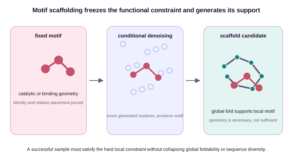
Imagine scaffolding a three-residue catalytic motif. The generator can place a compact fold around the residues while preserving their relative coordinates. Inverse folding can then assign a hydrophobic core and a polar pocket. A structure predictor may confirm that the resulting sequence returns to the designed geometry. Still, catalysis depends on protonation, solvent access, substrate pose, transition-state stabilization, and conformational motion. The scaffold has preserved a geometric hypothesis. It has not yet established the mechanism.
Distances alone do not preserve a coordination site
For the zinc motif, let \(d_i\) be the three metal–ligand distances and \(\phi_j\) the three pairwise angles around the metal. A dimensionless constraint score can use tolerances of 0.2 angstrom and 5 degrees:
\[C =\sum_{i=1}^{3} \left(\frac{d_i-d_i^\star}{0.2}\right)^2 +\sum_{j=1}^{3} \left(\frac{\phi_j-\phi_j^\star}{5}\right)^2.\]Candidate A has distances \((2.2,2.0,2.3)\) and angles \((112,109,110)\). Relative to the targets \((2.1,2.0,2.2)\) and \((110,108,109)\),
\[C_A =(0.5^2+0^2+0.5^2) +(0.4^2+0.2^2+0.2^2) =0.74.\]Candidate B has all three target distances exactly but angles \((90,129,108)\). Its angular contribution alone is
\[C_B =(-4)^2+(4.2)^2+(-0.2)^2 =33.68.\]A distance-only motif filter accepts both, although candidate B places the ligands in a different coordination geometry. A Cartesian motif RMSD can also hide chemically meaningful angular errors after averaging many atoms. The constraint should operate on the coordinating atoms and invariants that define the hypothesized mechanism, followed by side-chain, protonation, solvent, and energetic checks.
The distinction between a static design target and a distribution of functional conformations is developed in Protein Ensembles and Learned Molecular Dynamics. A motif that is perfectly arranged in one predicted structure can be too flexible, inaccessible, or populated too rarely in solution. Conversely, controlled flexibility may be required for binding or turnover. Static geometry is often the right starting constraint, but it is not the whole physical objective.
Co-Design Couples Discrete Chemistry and Continuous Geometry
The conventional pipeline first generates a backbone and then applies inverse folding. This factorizes a joint model as
\[p(a,X\mid y)=p(X\mid y)p(a\mid X,y).\]The factorization is attractive because each stage has a clear role and can use specialized training data. It also creates an interface failure: the backbone model may sample geometries in a region for which the sequence designer has little support. Repeating inverse folding with several sequences partly addresses this mismatch but does not change the backbone.
Joint or iterative co-design lets sequence and structure revise one another. One can alternate coordinate denoising with discrete residue updates, relax a continuous representation of sequence before discretization, or train a multimodal model over both. In principle this captures feedback: a glycine permits backbone angles that a bulky aromatic residue does not; a buried salt bridge changes which local packing arrangements are plausible. In practice the two spaces have different symmetries, noise processes, and error scales. Coordinates are continuous and equivariant under rigid motion; amino-acid identities are discrete and invariant. A single generation schedule can easily settle one variable before the other has enough information.
There is also a subtler issue. A joint model can make sequence and structure mutually consistent according to the same learned assumptions. This may improve internal scores without adding independent evidence. Coherence within a model is valuable, but it should not be mistaken for calibration against physical reality.
Exact factorization does not guarantee compatible learned stages
Any true joint distribution can be factorized as \(p(X)p(a\mid X)\), so sequential design is not mathematically less expressive by definition. The practical loss comes from training the two factors on different supports and then sampling them without feedback.
Partition backbone space into a sequence-designable region \(D\) and an incompatible region \(I\). Suppose the backbone generator assigns
\[p_\theta(D)=0.10, \qquad p_\theta(I)=0.90.\]The separately trained inverse folder produces a compatible sequence with probability 0.80 in \(D\) but only 0.01 in \(I\). The total proposal mass on compatible pairs is
\[0.10(0.80)+0.90(0.01)=0.089.\]Only 8.9% of sequential samples reach the compatible joint region. Generating ten sequences for every backbone does not fix the allocation cleanly: it spends most calls trying to rescue the 90% backbone mass in \(I\).
Suppose a joint or feedback-trained proposal shifts 0.60 probability mass directly onto compatible pairs in \(D\). Its useful proposal mass is then 0.60, about \(0.60/0.089\approx6.74\) times larger. That gain comes from changing the backbone proposal using sequence evidence, not from violating the probability factorization.
The reverse tradeoff is coverage. A joint model may concentrate on the easiest mutually predictable fold family and abandon unusual but physically viable scaffolds. Report valid pair mass together with backbone diversity, motif satisfaction, and novelty. Otherwise improved sequence–structure agreement may only show that both variables collapsed onto a shared familiar mode.
A Design Pipeline Is a Sequence of Falsification Attempts
In practice, generation is the first stage of a funnel. A backbone generator proposes geometries. An inverse-folding model supplies several sequences per backbone. A structure predictor refolds each sequence. Filters remove clashes, weak interfaces, exposed hydrophobics, poor confidence, undesirable motifs, or manufacturability risks. A much smaller set is synthesized and assayed.
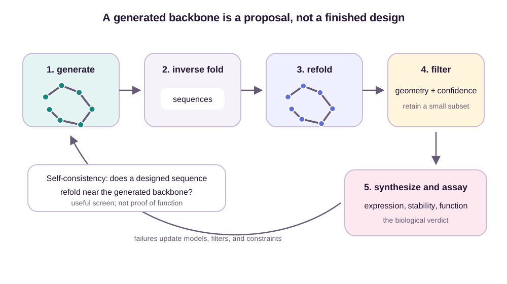
For a designed sequence \(a\) and target backbone \(X\), a common structural score compares a predicted fold \(\widehat X(a)\) with the target:
\[s_{\mathrm{sc}}(a,X) =\operatorname{sim}\!\left(\widehat X(a),X\right),\]using RMSD, TM-score, aligned error, or a combination. High self-consistency suggests designability: at least one sequence appears able to realize the generated backbone. It does not establish novelty, because a close database neighbor may already exist. It does not establish diversity, because thousands of samples may collapse to the same topology. And it does not establish function, because structure prediction is not an affinity or catalytic assay.
These axes must be reported separately:
- geometric validity: chain connectivity, bond geometry, clashes, chirality, and plausible secondary structure;
- designability: whether designed sequences independently refold to their intended backbones;
- diversity: how broadly samples cover sequence and structural space, rather than how many files were generated;
- novelty: distance to training and reference databases under sequence and structural search;
- constraint satisfaction: motif RMSD, interface geometry, symmetry, or other task-specific conditions;
- developability: expression, solubility, aggregation, immunogenicity, and manufacturability where relevant;
- experimental function: binding, activity, selectivity, kinetics, or cellular phenotype under a specified assay.
These objectives conflict. Lower-temperature sampling can raise average model likelihood while reducing diversity. Aggressive novelty thresholds can discard useful variations on known folds or push samples outside regions where predictors are calibrated. Tight motif constraints can reduce the number of globally foldable scaffolds. Selecting only the highest predicted affinity can enrich true binders while also magnifying oracle error. There is no scalar score that preserves every desirable property.
Agreement between learned models can be correlated evidence
Suppose the zinc-backbone generator and the refolding model both learned from overlapping Protein Data Bank structures, use related geometric representations, and favor compact helical bundles. From 100 generated designs, 60 pass the refolder’s self-consistency threshold. It is tempting to read the two models as independent votes.
Now apply an orthogonal physics-based calculation that includes metal coordination and protonation. Only 12 of the 60 retain a favorable zinc site after relaxation, and only 2 bind metal in experiment. The generator and refolder agreed because both recognized the same fold prior; neither was trained to resolve the missing coordination chemistry. Their agreement was internal self-consistency, not 60 independent confirmations of function.
Correlated failure can be more specific. Both models may reward a familiar histidine-rich pocket even when one histidine is protonated in a way that prevents coordination. A third learned model trained on similar structures can reproduce the same error. Model count is not evidence count when training data, representations, or physical assumptions overlap.
Validation should therefore name the independence level:
- internal consistency checks whether generated variables agree under the pipeline’s learned assumptions;
- orthogonal computation adds a different representation or physical model, such as explicit metal geometry, relaxation, or electronic scoring;
- experiment tests expression, folding, and metal binding in the specified assay.
Each level can reject candidates. Only the latter two add evidence not already encoded by the generator–refolder pair, and even orthogonal computation can share reference approximations with training labels.
The Experimental Denominator Matters
Suppose a model generates 10,000 backbones, 2,000 pass geometry filters, 300 obtain self-consistent sequences, 24 are selected by an affinity predictor, and 3 bind experimentally. “Three successful designs” is true. “A 12.5% hit rate” is also true for the selected set. Neither number estimates the probability that an unfiltered generator sample works, and neither reveals whether the affinity predictor improved selection unless appropriate controls were tested.
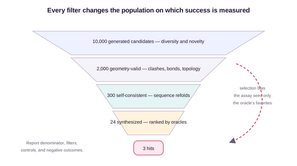
This is selection bias by construction. Wet-lab budgets require down-selection, but the resulting observations are concentrated where the pipeline already predicts success. Failed generated candidates are rarely synthesized, so the data cannot distinguish a strong generator from a strong filter applied to a weak generator. Even among synthesized designs, unsuccessful expression may prevent the intended functional assay, creating another conditional denominator.
A persuasive validation therefore reports the full funnel: how many candidates were generated, every filtering threshold, how many independent backbones and sequence clusters survived, what fraction was synthesized, and which assays each construct reached. Random or stratified controls can estimate the value of ranking. Near-neighbor baselines test whether novelty contributes anything beyond known scaffolds. Negative outcomes constrain the model just as importantly as positive structures. Prospective campaigns are strongest when the design and selection protocol is fixed before seeing assay results.
A stratified control estimates enrichment
Return to the hypothetical funnel: 10,000 generated backbones, 2,000 geometry-filtered backbones, and 300 self-consistent sequence–backbone pairs. Synthesize 24 constructs, but allocate them prospectively. Select 12 by the full affinity ranker. Select 12 uniformly across backbone clusters and motif-score strata among the other 288 candidates. The second arm is not an unfiltered generator control; it estimates the ranker’s value conditional on reaching the 300-candidate population.
Suppose the outcomes are:
| Arm | Synthesized | Solubly expressed | Folded among expressed | Metal binders among folded |
|---|---|---|---|---|
| Top-ranked | 12 | 9 | 7 | 3 |
| Stratified control | 12 | 8 | 5 | 1 |
The campaign-level binder yield is \(3/12=25.0\%\) for ranked designs and \(1/12=8.3\%\) for controls, a threefold observed enrichment. Conditional on reaching the binding assay, the rates are \(3/7=42.9\%\) and \(1/5=20.0\%\), a 2.14-fold enrichment. The first ratio includes expression and folding failures and is relevant to synthesis budget. The second isolates binding among folded proteins.
The sample is too small for a precise general claim: one additional control hit would double its campaign yield. The prespecified stratified allocation still creates a contemporaneous denominator for the selection rule under the same synthesis, expression, and assay conditions.
The upstream denominators remain visible. Ranked binders represent \(3/10{,}000=0.03\%\) of raw generated backbones only as a realized funnel yield. We cannot estimate the generator’s unfiltered success probability because 9,976 backbones were never assayed. Unsynthesized candidates are unobserved, not experimental failures.
Experimental evidence also has levels. Soluble expression is not proof of a monodisperse folded state. Circular dichroism reports secondary-structure content but not atomic accuracy. A crystal or cryo-EM structure can confirm the fold while leaving solution populations uncertain. Binding at one concentration does not establish affinity, specificity, or biological effect. The claim should stop where the assay stops.
Design Closes Only When Information Returns from the Lab
Generative models have changed protein design by making structural proposals abundant. Inverse folding can populate a proposed backbone with compatible sequences. Diffusion can complete a scaffold around a functional motif. Co-design can reduce the mismatch between discrete chemistry and continuous geometry. Predictors and learned oracles can compress a vast candidate set into an experimentally manageable one.
But abundance of proposals changes the bottleneck rather than removing it. The difficult question becomes which constraints deserve to enter generation, which independent models can reject failures, which tradeoffs should remain visible, and which experiments discriminate between a plausible molecular picture and the requested function. A successful protein-design system is therefore not a generator in isolation. It is a calibrated loop in which sequence, structure, and function remain distinct claims—and experimental outcomes return information to every stage that made them.
A feedback ledger assigns each failure
Across both experimental arms, 24 synthesized constructs yield 17 soluble proteins, 12 folded proteins, and 4 metal binders. Assign each non-hit to its earliest observed failure:
| Earliest failure | Count | Evidence updates | Next intervention |
|---|---|---|---|
| No soluble expression | 7 | Sequence/developability model and expression context | Redesign surface residues or expression construct |
| Expressed but not folded | 5 | Backbone designability and inverse-folding interface | Resample sequences or revise low-entropy scaffolds |
| Folded but no metal binding | 8 | Motif chemistry, accessibility, and functional ranker | Tighten orthogonal chemistry and assay-matched scores |
| Metal binding | 4 | Full pipeline under this assay | Measure affinity, selectivity, and structure |
A construct that never expresses does not provide a clean metal-binding measurement, so calling it a biochemical nonbinder confounds stages. A folded nonbinder is more informative about motif geometry and functional ranking than about inverse folding. The earliest-failure label makes negative data actionable.
The next campaign should preserve these stage labels. Retraining on all 20 failures with one binary outcome would erase why they failed. Backbone and inverse-folding components should learn from structural failures; expression models should learn from produced and soluble constructs; the functional oracle should learn from assay-qualified folded proteins. The stratified arm should remain large enough to tell whether a revised ranking policy enriches binders rather than merely reshuffling its own scores.
References
Madani, A. et al. “Large language models generate functional protein sequences across diverse families.” Nature Biotechnology 41, 1099–1106 (2023). doi:10.1038/s41587-022-01618-2 ↩
Dauparas, J. et al. “Robust deep learning-based protein sequence design using ProteinMPNN.” Science 378, 49–56 (2022). doi:10.1126/science.add2187 ↩
Watson, J. L. et al. “De novo design of protein structure and function with RFdiffusion.” Nature 620, 1089–1100 (2023). doi:10.1038/s41586-023-06415-8 ↩
Ingraham, J. B. et al. “Illuminating protein space with a programmable generative model.” Nature 623, 1070–1078 (2023). doi:10.1038/s41586-023-06728-8 ↩
Figure provenance: all four diagrams are original explanatory syntheses created for this post with scripts/generate_protdesign_figures.py. They use no copied slide, paper, or Flaticon assets and are released under CC BY 4.0 with the post.