On this page
Adapted from my 2025 Geometric Deep Learning and Machine Learning for Molecules lectures. The central question is whether a structural representation is sufficient to serve as a dynamical state, linking equilibrium weights, coarse transfer operators, and physical-time path laws. For trajectory mechanics and error budgets, see Molecular Simulation with Machine-Learned Force Fields.
A protein structure is not a single object. Even at fixed sequence, solvent, temperature, protonation, and binding partners, the atoms fluctuate. Flexible loops move, side chains exchange rotamers, domains open and close, and disordered regions occupy broad families of conformations. Some states exchange in picoseconds; others remain separated for milliseconds or longer.
This makes “predict the structure distribution” ambiguous. An equilibrium model should reproduce how often each conformation occurs. A dynamical model should additionally reproduce how conformations are connected and how long transitions take. A set of beautiful structures can satisfy the first criterion badly and the second criterion not at all.
The distinction matters for learned models. A diffusion or flow model can draw independent equilibrium-like structures without defining physical time. A transfer model can predict a future state at a chosen lag. A trajectory generator can synthesize an entire path. These objects answer different scientific questions, require different training data, and demand different validation.
Metastable states organize a protein ensemble
Let \(x\) denote all molecular coordinates after fixing the thermodynamic system and removing irrelevant rigid motion. At temperature \(T\), the canonical equilibrium density is
\[\mu(x) =\frac{1}{Z}\exp[-\beta U(x)], \qquad \beta=(k_{\mathrm B}T)^{-1},\]where \(U(x)\) is the potential energy and \(Z\) is the partition function. A low-dimensional collective variable \(z=\xi(x)\)—a torsion, contact pattern, inter-domain distance, or learned coordinate—induces the marginal
\[p(z) =\int \mu(x)\,\delta(z-\xi(x))\,dx.\]Its free energy is
\[F(z) =-k_{\mathrm B}T\log p(z)+C.\]Basins of \(F\) correspond to frequently occupied conformational families. High barriers separate metastable states: the system mixes rapidly inside a state but leaves it rarely. The protein therefore has two scales at once—fast local fluctuations and slow state exchange.
We will follow one protein switch through the chapter. States \(A_1\) and \(A_2\) are geometrically similar open conformations with different side-chain rotamers; state \(B\) is closed. At a lag \(\tau=10\) ns, suppose the microstate transition matrix is
\[\mathbf T= \begin{pmatrix} 0.90&0.09&0.01\\ 0.09&0.71&0.20\\ 0.01&0.20&0.79 \end{pmatrix}.\]Rows are source states and columns are destination states, in the order \((A_1,A_2,B)\). Every entry is nonnegative and every row sums to one. The matrix is symmetric, so its stationary distribution is immediately
\[\boldsymbol\pi =\left(\frac13,\frac13,\frac13\right), \qquad \boldsymbol\pi\mathbf T=\boldsymbol\pi.\]The two open rotamers together have equilibrium probability \(\pi_O=2/3\), while the closed state has \(\pi_B=1/3\). Aggregating their equilibrium weights gives
\[F_B-F_O =-k_{\mathrm B}T\log\frac{\pi_B}{\pi_O} =k_{\mathrm B}T\log2 \approx0.693\,k_{\mathrm B}T.\]The closed basin is therefore higher in aggregate free energy even though every microstate has equal stationary weight. State degeneracy matters: merging two equally populated open rotamers doubles the open basin’s probability. The same merge will fail for dynamics because \(A_1\) and \(A_2\) do not have the same exit law.
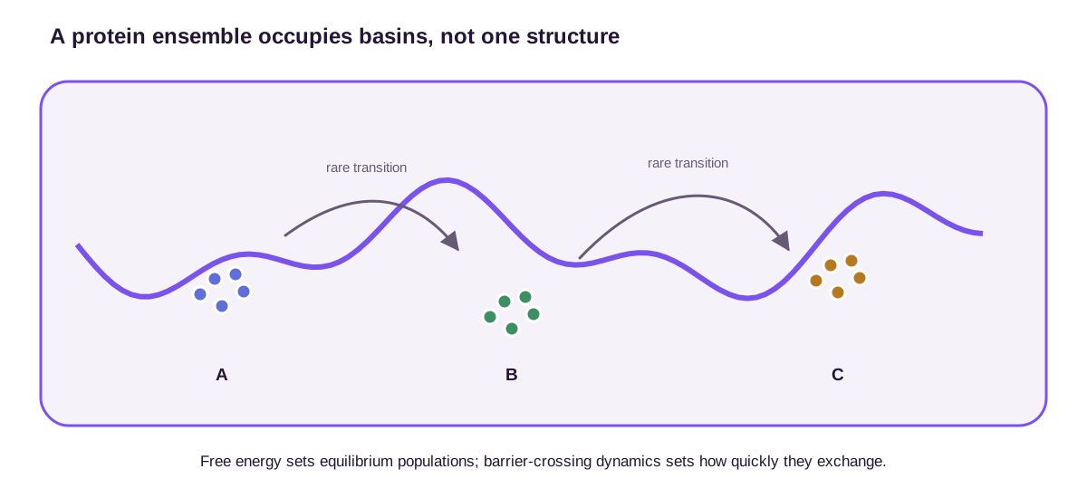
Free energy alone does not determine kinetics. Two systems can share \(p(z)\) but have different diffusivity along \(z\), different hidden barriers orthogonal to \(z\), and different transition mechanisms. Projecting onto a poor collective variable can even make a non-Markovian process look like motion on a simple landscape.
This is the first recurring warning: a landscape is a marginal description, not a literal track on which a protein moves.
Molecular dynamics supplies both ensembles and time order
Molecular dynamics integrates forces from a molecular Hamiltonian or machine-learned potential. With a thermostat, a sufficiently long and ergodic trajectory can sample an equilibrium ensemble. Unlike an unordered structural dataset, the trajectory also records temporal correlations and transition pathways.
The molecular-simulation post develops initialization, integration, force-field error, and ensemble validation. Here the central limitation is timescale separation. A femtosecond step is needed to resolve fast atomic motion, while a biologically interesting conformational change may take milliseconds. One event can require roughly a trillion integration steps.
The running model makes the scale explicit. With a \(2\) fs integration step, one \(10\) ns MSM lag contains
\[\frac{10\ \mathrm{ns}}{2\ \mathrm{fs}} =5\times10^6\]force evaluations. A \(1\) microsecond trajectory contains \(5\times10^8\) steps but only 100 nonoverlapping 10-ns blocks. Saving coordinates every picosecond produces a million frames, not a million independent observations of the slow switch. Integrator resolution, stored-frame count, and transition-scale sample size are three different clocks.
Running many shorter trajectories in parallel improves coverage, especially when seeded from diverse states, but it does not automatically solve rare-event sampling. Enhanced-sampling methods deliberately alter exploration. Replica exchange changes temperature or Hamiltonian across replicas. Umbrella sampling restrains chosen collective variables. Metadynamics deposits a history-dependent bias that discourages revisiting explored regions (Laio & Parrinello, 2002).
Biased samples cannot be treated as ordinary equilibrium frames. Recovering unbiased populations requires the method’s reweighting formula and adequate overlap. Kinetics is even more delicate: a bias that accelerates barrier crossing usually changes physical transition times. Enhanced sampling may give a reliable free-energy difference while destroying the natural path timing.
Suppose an enhanced-sampling bias lowers state \(B\) by \(k_{\mathrm B}T\log4\) and leaves \(A_1,A_2\) unchanged. Starting from the uniform target, the biased probabilities are proportional to \((1,1,4)\). An exact 600-frame sample then contains counts \((100,100,400)\). Raw counting reports closed probability \(2/3\) rather than \(1/3\). The unbiased importance factor is proportional to \(e^{\beta V}\), so frames in \(B\) receive weight \(1/4\) and open frames receive weight 1. The weighted totals become \((100,100,100)\) and recover the uniform microstate distribution.
Reweighting restores this equilibrium statistic under the assumed bias and overlap; it does not restore the 10-ns transition matrix. The effective sample size of the weighted frames is
\[M_{\mathrm{eff}} =\frac{\left(\sum_m w_m\right)^2}{\sum_m w_m^2} =\frac{300^2}{100+100+400/16} =400.\]The bias produced 600 stored frames but only 400 weight-equivalent samples. Time correlation would reduce the effective size further.
The force field remains another source of uncertainty. A perfectly converged simulation samples the equilibrium distribution of its chosen Hamiltonian, which may disagree with the real protein because of water balance, ion parameters, protonation, polarization, or missing chemistry. Longer sampling removes statistical error but not Hamiltonian bias.
Markov state models compress long-time kinetics
A Markov state model partitions configuration space into states \(S_1,\ldots,S_K\) and estimates transition probabilities at lag time \(\tau\):
\[T_{ij}(\tau) =\Pr(X_{t+\tau}\in S_j\mid X_t\in S_i).\]Given transition counts \(C_{ij}(\tau)\), the simplest estimator normalizes rows,
\[\widehat T_{ij} =\frac{C_{ij}}{\sum_j C_{ij}},\]although reversible and Bayesian estimators are often preferable. The stationary distribution satisfies
\[\boldsymbol{\pi}^{\mathsf T}T =\boldsymbol{\pi}^{\mathsf T}.\]At equilibrium, detailed balance is
\[\pi_iT_{ij} =\pi_jT_{ji}.\]The nontrivial eigenvalues \(1>\lambda_2\geq\lambda_3\geq\cdots\) encode relaxation times,
\[t_k =-\frac{\tau}{\log |\lambda_k|}.\]Thus one compact object provides state populations, slow timescales, and transition-path statistics. Prinz et al. develop the construction and its validation in detail (Prinz et al., 2011).
For the running chain, an exact finite count matrix with 1,000 outgoing transitions from each state is
\[\mathbf C= \begin{pmatrix} 900&90&10\\ 90&710&200\\ 10&200&790 \end{pmatrix}.\]Row normalization recovers \(\mathbf T\) exactly. The counts are symmetric, so the observed flux from \(i\) to \(j\) equals the reverse flux. With \(\pi_i=1/3\),
\[\pi_iT_{ij}=\frac13T_{ij} =\frac13T_{ji}=\pi_jT_{ji},\]which verifies detailed balance for every pair. Symmetry is sufficient here because the stationary weights are uniform; a reversible chain with nonuniform weights need not have a symmetric transition matrix.
The eigenvalues are
\[\lambda_1=1, \qquad \lambda_2\approx0.865227, \qquad \lambda_3\approx0.534773.\]At \(\tau=10\) ns, the implied timescales are
\[t_2=-\frac{10}{\log0.865227}\approx69.1\ \mathrm{ns}, \qquad t_3=-\frac{10}{\log0.534773}\approx16.0\ \mathrm{ns}.\]These are relaxation times of ensemble modes, not mean dwell times of a named state. The unit eigenvalue carries the stationary distribution; the two decaying modes describe how deviations from equilibrium disappear.
The exact count table is deliberately clean. With finite independent transitions, the row-wise standard error for a binomial entry is approximately \(\sqrt{T_{ij}(1-T_{ij})/N_i}\). For 1,000 transitions from each source, this is about \(0.00315\) for \(A_1\to B\) and \(0.01265\) for \(A_2\to B\). Their difference of \(0.19\) is far larger than either counting scale. Molecular transition counts are usually correlated and reversible estimators couple entries, so trajectory blocks or posterior intervals should replace this naive calculation in practice. The finite calculation only shows that sampling uncertainty and state-definition error are separate budgets.
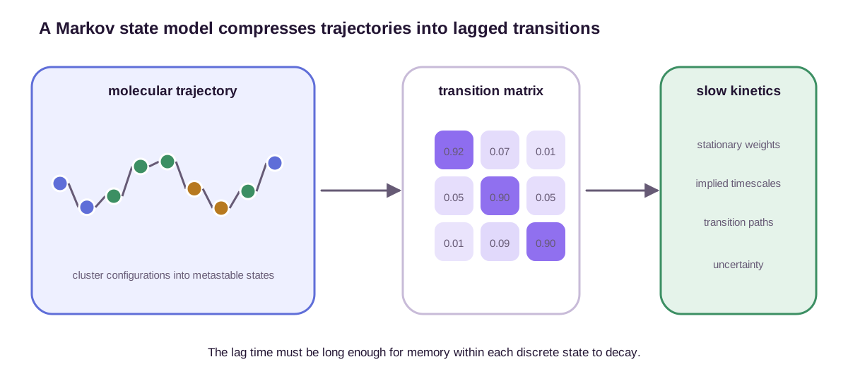
The Markov approximation is not automatic. If a state combines configurations that relax slowly relative to \(\tau\), the next-state distribution retains memory of where the trajectory entered. Increasing \(\tau\) reduces this memory but discards temporal resolution and reduces the number of observed transitions. Implied timescales should plateau across a range of lag times, and Chapman–Kolmogorov tests should compare multi-step predictions \(T(\tau)^n\) with directly observed transitions at \(n\tau\).
Clustering geometry is equally consequential. RMSD may split a kinetically coherent basin or merge distinct states separated by a hidden barrier. A useful representation emphasizes slow coordinates rather than merely large geometric variance.
The proposed open state \(O=\{A_1,A_2\}\) is a concrete bad merge. A partition is strongly lumpable when every microstate inside a macrostate has the same total probability of entering each macrostate. Here
\[P(B\mid A_1)=0.01, \qquad P(B\mid A_2)=0.20.\]The two geometrically similar rotamers differ twentyfold in their chance of closing over one lag. No single open-to-closed transition probability can represent both initial conditions.
At equilibrium, conditioning on being open gives the hidden mixture \((1/2,1/2)\) over \((A_1,A_2)\). Averaging with that particular mixture produces
\[\mathbf T_{\mathrm{eq}}^{O/B} = \begin{pmatrix} 0.895&0.105\\ 0.210&0.790 \end{pmatrix}.\]This two-state matrix has stationary weights \((2/3,1/3)\) and satisfies coarse detailed balance because \((2/3)(0.105)=(1/3)(0.210)=0.07\). It correctly predicts one coarse step when the hidden open rotamer is equilibrium-conditioned. Those successes do not make the projected process Markov.
History changes the hidden mixture. Immediately after a transition from \(B\) into \(O\), the probabilities of landing in \(A_1\) and \(A_2\) are proportional to \(T_{BA_1}=0.01\) and \(T_{BA_2}=0.20\). Thus
\[P(A_1\mid B\to O)=\frac1{21}, \qquad P(A_2\mid B\to O)=\frac{20}{21}.\]The probability of closing again on the next lag is then
\[\frac1{21}(0.01) +\frac{20}{21}(0.20) \approx0.19095,\]not the equilibrium-conditioned value \(0.105\). The observed macrostate is \(O\) in both cases, yet knowledge that the chain just entered from \(B\) nearly doubles the next closing probability. The missing rotamer stores memory.
A Chapman–Kolmogorov calculation exposes the same failure without conditioning on an entry event. Squaring the equilibrium-conditioned coarse matrix gives
\[\left[\left(\mathbf T_{\mathrm{eq}}^{O/B}\right)^2\right]_{OB} =0.176925.\]Directly propagating the equilibrium open mixture through the microstate matrix for two lags gives
\[\frac12 \left[(\mathbf T^2)_{A_1B}+(\mathbf T^2)_{A_2B}\right] =\frac12(0.0349+0.3009) =0.1679.\]The discrepancy is exact, not sampling noise. Keeping \(A_1\) and \(A_2\) separate restores a Markov description for this chain. A history label such as “newly entered open” can also repair prediction at the cost of a larger state. Increasing lag may allow the rotamer mixture to relax before the next observation, but that is an empirical approximation: implied timescales and Chapman–Kolmogorov errors must stabilize at the chosen lag.
Even survival inside \(O\) changes the hidden mixture. Starting from the equilibrium mixture, one open-to-open step leaves unnormalized weights \((0.495,0.400)\) and therefore conditional mixture \((0.553,0.447)\). Its next closing probability falls to about \(0.0949\). Starting from the entry-conditioned mixture \((1/21,20/21)\), one surviving open step gives conditional mixture \((0.159,0.841)\) and next closing probability \(0.1698\). The apparent hazard depends on how long the process has been open and how it entered.
The equilibrium-conditioned coarse matrix has nontrivial eigenvalue \(0.685\), corresponding to implied time \(-10/\log0.685\approx26.4\) ns. Neither microstate timescale, \(69.1\) ns or \(16.0\) ns, equals that value. Aggregation has mixed the two relaxation modes into a history-dependent process; fitting one exponential supplies a convenient summary, not an exact retained mode.
Learned latent dynamics search for slow coordinates
Traditional pipelines choose molecular features, perform a time-lagged dimensional reduction, cluster, and estimate transitions. Learned latent models replace some or all of these steps with a neural encoder
\[z_t=f_\theta(x_t).\]A reconstruction objective alone tends to preserve coordinates that explain structural variance, which need not be kinetically slow. Time-lagged objectives instead reward representations that predict \(x_{t+\tau}\) or approximate the leading singular functions of the transfer operator.
VAMPnets learn soft state memberships and a kinetic model end to end using a variational score for Markov processes (Mardt et al., 2018). Their latent states are optimized for slow dynamics rather than visual separation. Related time-lagged autoencoders, Koopman models, and neural transfer operators learn a coordinate system in which long-time evolution is approximately linear or easier to propagate.
This compression can pool many short trajectories into estimates of slow behavior. It cannot infer unobserved mechanisms without assumptions. If no trajectory crosses between two basins, a learned transition rate is extrapolation. A model may infer a plausible bridge from related proteins or structural priors, but the evidence is no longer contained in the trajectory data alone.
Protein generalization adds a second challenge. A latent coordinate learned for one sequence may describe a particular loop motion; the analogous functional coordinate in another protein can involve different residues. Sequence-conditioned geometric encoders must align these motions without erasing protein-specific states.
In the three-state switch, an encoder trained mainly on coordinate reconstruction may map \(A_1\) and \(A_2\) to one compact open cluster because their backbones are nearly identical. Once the decoder exposes only \(O\), no downstream memoryless transition network can return both \(0.01\) and \(0.20\) for the same encoded input. This collision holds for every parameter choice of that downstream model. A time-lagged objective can separate the rotamers if their different futures are present in training, but the representation must retain the side-chain or history variable that makes those futures distinguishable.
Equilibrium generators skip the physical path
An equilibrium generator aims to draw independent samples from \(\mu(x)\). Boltzmann generators use invertible flows to map a simple latent distribution into molecular configurations and correct the generated distribution with statistical-mechanical weights (Noé et al., 2019). If samples are independent, they can cross free-energy barriers without waiting for local dynamics.
Diffusion and flow models extend this strategy to flexible geometric architectures. AlphaFlow repurposes a protein structure predictor inside a flow-matching framework and learns sequence-conditioned ensemble variation from structural and molecular-dynamics data (Jing et al., 2024). The model can generate a diverse ensemble much faster than integrating atomistic dynamics for the same number of decorrelated frames.
The geometric flow post explains how translations, rotations, and internal geometry constrain these paths. For proteins, rigid residue frames or backbone coordinates must transform equivariantly, while the output density remains invariant to a global laboratory frame.
Independent ensemble samples are valuable for equilibrium observables:
\[\langle A\rangle_\mu =\int A(x)\mu(x)\,dx \approx\frac{1}{M}\sum_{m=1}^M A(x^{(m)}).\]That unweighted average is valid only when the generator samples \(\mu\) exactly. Suppose a generator instead proposes state probabilities
\[q=(0.10,0.40,0.50)\]and returns exact counts \((100,400,500)\) in 1,000 independent samples. The target remains \(\mu=(1/3,1/3,1/3)\). Importance weights \(w_i=\mu_i/q_i\) are therefore \(10/3,5/6,2/3\). Each state’s total weight is \(1000/3\), so the weighted closed-state indicator recovers \(1/3\) rather than the raw \(1/2\).
The correction has a variance cost. Its effective sample size is
\[M_{\mathrm{eff}} =\frac{(\sum_m w_m)^2}{\sum_m w_m^2} =\frac{1000^2} {100(10/3)^2+400(5/6)^2+500(2/3)^2} \approx621.\]This calculation assumes the target-to-proposal density ratio is known and that \(q\) covers every target state. If the generator never produces \(A_1\), no finite weight can recover its contribution. Structural diversity and valid importance weights are separate requirements.
But the denoising or flow time used to generate \(x^{(m)}\) is an algorithmic coordinate, not physical time. A path from Gaussian noise to a folded structure does not describe how the protein folds. Equilibrium generation can answer “which conformations and with what weights?” without answering “how do they interconvert?”
Trajectory generators model ordered paths
A dynamical surrogate instead models a transition kernel,
\[p_\theta(x_{t+\Delta}\mid x_t),\]or a joint path distribution conditioned on endpoints or partial frames. Autoregressive transition models repeatedly sample the next coarse time step. Conditional normalizing flows can learn large-lag transfer operators. Diffusion and flow models can treat a trajectory as a geometric time series and generate many frames jointly.
MDGen demonstrates the joint-trajectory view for forward simulation, endpoint-conditioned transition paths, temporal upsampling, and inpainting (Jing et al., 2024). Joint generation reduces the accumulation of one-step errors and permits noncausal conditioning. It also creates a harder consistency problem: the sampled path must be geometrically valid at every frame and statistically compatible across time.
Multi-lag consistency is an executable version of that requirement. Suppose a learned open/closed model predicts at 10 ns
\[\widehat{\mathbf P}_{10} = \begin{pmatrix}0.90&0.10\\0.10&0.90\end{pmatrix},\]but a separately trained 20-ns head predicts
\[\widehat{\mathbf P}_{20} = \begin{pmatrix}0.75&0.25\\0.25&0.75\end{pmatrix}.\]Both matrices are valid, reversible, and stationary at \((1/2,1/2)\). A time-homogeneous Markov process would require the semigroup relation
\[\mathbf P_{20}=\mathbf P_{10}^2 = \begin{pmatrix}0.82&0.18\\0.18&0.82\end{pmatrix},\]which the learned heads violate by \(0.07\) in every entry. Their implied timescales also disagree: \(-10/\log0.8\approx44.8\) ns versus \(-20/\log0.5\approx28.9\) ns. Accurate held-out likelihood at each lag does not guarantee that the heads describe one physical clock. Joint training, an explicit generator, or a semigroup penalty can reduce the inconsistency; held-out multi-step propagation must still test it.
Conditioning is scientifically useful. Given two metastable endpoints, a model can propose transition paths. Given sparse experimental restraints, it can generate compatible ensembles. Given the trajectory of one protein region, it can inpaint coupled motion elsewhere. But conditioning changes the target distribution. Endpoint-conditioned transition paths are rare-event bridges, not ordinary equilibrium trajectories; property-guided samples need correction before being interpreted as unbiased populations.
Equilibrium and kinetics can disagree completely
Consider two states \(A\) and \(B\) with stationary probabilities \(\pi_A=\pi_B=1/2\). A reference process might have rates
\[k_{A\to B}=k_{B\to A}=10^{-3}\ \mathrm{ns}^{-1},\]while a surrogate uses
\[\widetilde k_{A\to B} =\widetilde k_{B\to A} =1\ \mathrm{ns}^{-1}.\]Both satisfy detailed balance and have the same equilibrium distribution. Their relaxation times differ by a factor of one thousand. A snapshot-based metric cannot tell them apart.
The full transition kernel makes the clock visible. For symmetric rate \(k\) and row-vector convention, the continuous-time generator is
\[\mathbf Q_k = \begin{pmatrix}-k&k\\k&-k\end{pmatrix}, \qquad \mathbf P_k(t)=e^{t\mathbf Q_k}.\]Rows of \(\mathbf Q_k\) sum to zero, its off-diagonal entries are nonnegative, and \((1/2,1/2)\mathbf Q_k=0\). Diagonalizing into the stationary vector \((1,1)\) and difference vector \((1,-1)\) gives
\[\mathbf P_k(t) =\frac12 \begin{pmatrix} 1+e^{-2kt}&1-e^{-2kt}\\ 1-e^{-2kt}&1+e^{-2kt} \end{pmatrix}.\]The difference mode decays as \(e^{-2kt}\), so the relaxation time is \(t_{\mathrm{relax}}=1/(2k)\). The reference rate \(10^{-3}\ \mathrm{ns}^{-1}\) gives \(500\) ns; the surrogate rate \(1\ \mathrm{ns}^{-1}\) gives \(0.5\) ns. At one nanosecond their switching probabilities are approximately
\[P_{A\to B}^{\mathrm{slow}}(1) =\frac{1-e^{-0.002}}2 \approx0.0010, \qquad P_{A\to B}^{\mathrm{fast}}(1) =\frac{1-e^{-2}}2 \approx0.4323.\]Both kernels approach the same stationary distribution as \(t\to\infty\). Equilibrium agreement erases the factor of one thousand because it sees only the zero eigenmode of the generator.
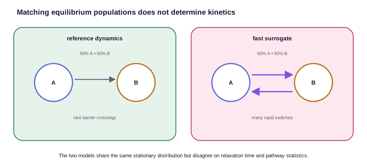
The reverse failure also occurs. A local transition model can predict short-time fluctuations accurately while drifting toward the wrong stationary distribution after repeated rollout. Enforcing detailed balance or training against equilibrium data can help, but consistency must be tested rather than assumed.
This yields a clean hierarchy. An ensemble model needs the correct stationary distribution. A transfer model needs the correct conditional distribution at its specified lag and the correct stationary distribution under iteration. A physical-time trajectory model additionally needs multi-time correlations, pathway statistics, and calibrated time units.
Validation must match the scientific claim
Structural plausibility is the first gate: bond geometry, stereochemistry, excluded volume, secondary structure, and global frame symmetry. A generated backbone can have good RMSD while containing local clashes or unrealistic peptide geometry.
Equilibrium validation compares state populations, free-energy differences, contact and distance distributions, radius of gyration, solvent exposure, and higher-order correlations. Coverage and precision must both be reported. A broad model can cover every reference state by producing many unphysical structures; a sharp model can look precise while missing rare functional basins.
Kinetic validation compares implied timescales, autocorrelation functions, mean first-passage times, transition-path ensembles, committor statistics, and Chapman–Kolmogorov consistency. Evaluation should use held-out temporal blocks or independent trajectories, not random frames from the same correlated run.
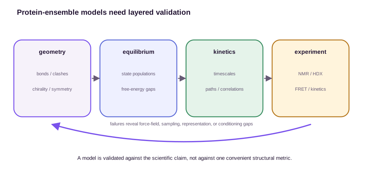
Experimental observables are ensemble averages filtered through a measurement model. NMR chemical shifts and order parameters, hydrogen–deuterium exchange, single-molecule FRET, SAXS, cryo-EM heterogeneity, and kinetic rate measurements each see different aspects of the ensemble. Agreement with one observable does not uniquely identify the full distribution. Forward models from structure to experiment have their own uncertainty, and several ensembles may fit the same low-dimensional measurement.
The forward map is often nonlinear, so evaluating it on an average structure is incorrect. For a simple FRET model with Förster radius \(R_0=5\) nm,
\[E(r)=\frac{1}{1+(r/R_0)^6}.\]Suppose an ensemble has half its weight at donor–acceptor distance \(3\) nm and half at \(7\) nm. The measured ensemble average is
\[\langle E\rangle =\frac12\left[E(3)+E(7)\right] =\frac12(0.9554+0.1172) \approx0.5363.\]The mean distance is \(5\) nm, but \(E(\langle r\rangle)=E(5)=0.5\). The two operations differ because \(E\) is nonlinear. Agreement should compare the average of the forward model over generated structures with the experimental observable, while propagating uncertainty in distances, dye linkers, and the forward model itself.
One average also remains nonidentifying even with an exact forward model. A single-distance ensemble concentrated near \(r=4.88\) nm has \(E(r)\approx0.5363\), matching the bimodal 3/7-nm ensemble above while having zero distance variance. Mean FRET cannot distinguish them. An efficiency distribution, another labeling geometry, or a complementary observable can constrain the missing heterogeneity; none turns one scalar average into a unique ensemble.
Forward-model validation must therefore declare both the measured random variable and its aggregation. Matching a population mean supports that mean under the stated labeling model; it does not validate state populations, transition rates, or individual structural assignments that the measurement integrated out.
The validation target can now be stated without using “realistic dynamics” as a catch-all:
| Scientific claim | Mathematical object required | Matched diagnostic | Failure that can still remain |
|---|---|---|---|
| Plausible structures | Supported conformations and local geometry | Stereochemistry, clashes, coverage and precision | Wrong state weights |
| Equilibrium ensemble | Stationary distribution \(\mu\) | State populations, reweighted observables, free energies, ESS | Wrong transition law |
| Transfer at lag \(\tau\) | Kernel \(T(\tau)\) on a declared state | Held-out transition counts and likelihood | Multi-lag inconsistency |
| Markov coarse dynamics | Lumpable or approximately Markov state representation | Entry-history comparison, implied-time plateau, Chapman–Kolmogorov test | Hidden memory outside tested lags |
| Physical-time paths | Consistent finite-dimensional path laws with calibrated clock | Autocorrelations, rates, first-passage and path statistics | Force-field or protocol bias shared by reference |
| Experimental prediction | Ensemble plus named forward model | Prospective complementary observables not used for conditioning | Nonidentifiability and forward-model error |
The strongest test combines complementary observables and predicts data not used for conditioning. If experimental restraints were supplied to the generator, reproducing them is a constraint-satisfaction check, not independent validation.
Failure modes are usually category errors
Several recurring failures follow directly from confusing the target objects:
- Flow time is treated as physical time. A generative path is interpreted as a folding trajectory without kinetic calibration.
- Diversity is mistaken for equilibrium weight. Many distinct structures are generated, but their frequencies do not follow the desired ensemble.
- Biased simulation is treated as unbiased data. Enhanced-sampling frames train a model without reweighting or labeling the bias.
- Random-frame splitting leaks trajectories. Near-duplicate temporal neighbors appear in both training and test sets.
- A learned state hides memory. The latent partition looks compact but fails lag-time and Chapman–Kolmogorov tests.
- Protein-level generalization is overstated. Homologous sequences or nearly identical folds cross the split boundary.
- Force-field truth is confused with experimental truth. A model perfectly emulates a simulation whose Hamiltonian is systematically wrong.
The three-state switch turns that list into a diagnosis. A generator that returns one third \(A_1\), one third \(A_2\), and one third \(B\) passes the stationary-population test. If the samples are independent, their order contains no estimate of \(\mathbf T\). Randomly shuffling them and counting adjacent labels would create an artificial kernel with every row equal to \(\boldsymbol\pi\). That kernel has the correct equilibrium distribution and erases both physical timescales.
A trajectory model can fail in a different order. It may reproduce the 10-ns count matrix on held-out transitions yet violate the 20-ns semigroup relation. That result supports interpolation of one conditional kernel, not a physical-time process. If the same model first merges \(A_1\) and \(A_2\), its failure is upstream: no memoryless coarse kernel can reproduce the microstate dynamics for all histories. More trajectory data can shrink uncertainty around the equilibrium-conditioned value \(0.105\) without making that value correct for a newly entered open state.
Each failure has a matched intervention. Wrong equilibrium weights call for reweighting, broader support, or a corrected energy model. Semigroup failure calls for joint multi-lag training or an explicit continuous-time generator. Hidden-state memory calls for state refinement, a longer validated lag, or an explicit history variable. Numerical instability calls for solver refinement. Experimental disagreement calls for auditing both the ensemble and the named forward model. Applying one remedy everywhere can make the diagnosis worse: increasing lag may reduce hidden memory while discarding short-time kinetics, and stronger enhanced sampling may improve weights while further corrupting raw transition times.
Data splitting follows the same claim. Random frames test interpolation among temporal neighbors. Held-out contiguous trajectory blocks test short-horizon rollout under familiar proteins and conditions. Independent simulation seeds test sensitivity to initialization. Holding out entire proteins tests sequence transfer, provided homologous and near-identical structural families do not cross the boundary. Experimental validation adds a different reference rather than another split of the same force-field trajectory.
Uncertainty should be decomposed accordingly: finite sampling, force-field error, generative-model error, state-discretization error, and experimental forward-model error are not interchangeable confidence intervals.
Proteins are ensembles because thermal motion and competing interactions populate many conformations. They exhibit dynamics because those conformations are connected by structured, often rare transitions. Learned models can accelerate both tasks, but only if the distinction remains explicit. An equilibrium generator may leap between basins and still be scientifically valid. A kinetic model must earn the right to attach a clock to those leaps.
References
- Laio, A., & Parrinello, M. (2002). Escaping free-energy minima. Proceedings of the National Academy of Sciences, 99(20), 12562–12566. ↩
- Prinz, J.-H., Wu, H., Sarich, M., Keller, B., Senne, M., Held, M., Chodera, J. D., Schütte, C., & Noé, F. (2011). Markov models of molecular kinetics: Generation and validation. The Journal of Chemical Physics, 134, 174105. ↩
- Mardt, A., Pasquali, L., Wu, H., & Noé, F. (2018). VAMPnets for deep learning of molecular kinetics. Nature Communications, 9, 5. ↩
- Noé, F., Olsson, S., Köhler, J., & Wu, H. (2019). Boltzmann generators: Sampling equilibrium states of many-body systems with deep learning. Science, 365(6457), eaaw1147. ↩
- Jing, B., Berger, B., & Jaakkola, T. (2024). AlphaFold meets flow matching for generating protein ensembles. Proceedings of the 41st International Conference on Machine Learning, 22277–22303. ↩
- Jing, B., Stärk, H., Jaakkola, T., & Berger, B. (2024). Generative modeling of molecular dynamics trajectories. Advances in Neural Information Processing Systems, 37. ↩
Figure provenance. All four protens_ diagrams are original SVG illustrations generated by scripts/generate_protens_figures.py. They synthesize standard statistical-mechanical and kinetic-modeling concepts described in the cited primary literature; no third-party artwork is reproduced.