Protein Design

Note: This post is written for ML researchers entering the protein design field. It covers the structural biology you need to read RFDiffusion and ProteinMPNN papers, understand what pLDDT and ipTM measure, and follow a design project from target definition through experimental validation. No biology background is assumed.

Introduction

Protein binders can contact broad target surfaces that are difficult to address with a small molecule. Their larger interfaces offer more geometric and chemical interactions to design, but size alone does not guarantee selectivity. Delivery, stability, and off-target binding remain part of the problem.

Structure-guided design has produced experimentally useful proteins. Hsieh and colleagues engineered a stabilized prefusion SARS-CoV-2 spike immunogen (Hsieh et al., 2020), while designed miniprotein inhibitors achieved picomolar binding to the spike in laboratory assays (Cao et al., 2020). These examples establish particular designs under particular assays, not a general success rate for protein design.

For ML researchers, the appeal is structural. Protein design is a well-defined generative modeling problem: the input is a functional specification (target structure, binding constraints), and the output is a sequence of discrete tokens (amino acids) that must satisfy continuous geometric constraints (3D folding).

Training draws on experimentally determined structures in the Protein Data Bank and much larger sequence collections. Structure predictors such as AlphaFold provide computational screens for candidate designs, not an experimental oracle: agreement with a predicted fold does not establish expression, binding, or function.

Rosetta established a design workflow based on energy functions and conformational search. AlphaFold2, ProteinMPNN, and RFdiffusion introduced learned models for structure prediction, inverse folding, and backbone generation. These tools can reduce computational cost and support experimentally successful campaigns, but hit rates depend on the target, design protocol, filters, and assay. Comparing percentages across campaigns requires matching those conditions and their denominators.

The background splits into two parts: the biology and the computational infrastructure around it.

Overview

A modern design campaign is a pipeline: RFDiffusion generates candidate backbone structures conditioned on the target, ProteinMPNN designs amino acid sequences for each backbone, AlphaFold predicts whether each sequence folds as intended, and the top candidates go to the lab. The numerical funnel later in this post is an illustrative campaign, not a reported benchmark.

The biology explains why each step works and fails: what proteins are made of, what forces hold the shape together, what makes a good binding interface, and what physical constraints the pipeline must satisfy. The organizing frame is the sequence → structure → function triangle.

What a Protein Is

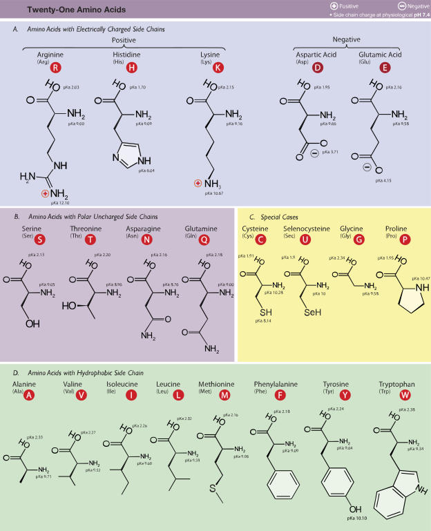
A protein is a chain of amino acids, small molecules linked end-to-end like beads on a string. There are 20 standard types, each identified by a one-letter code (A for alanine, M for methionine, etc.), so a protein sequence reads like MKVLWAGG...: a string over a 20-letter alphabet.

Every amino acid shares the same backbone atoms — a repeating N-C\(_\alpha\)-C unit — but differs in its side chain, the group that branches off at each C\(_\alpha\). Side chains vary in size, charge, and hydrophobicity.¹ This chemical diversity gives proteins their functional range.

Structure Hierarchy

Proteins organize at four levels:

1. Primary structure — the amino acid sequence itself.
2. Secondary structure — local repeating patterns. Alpha helices are coiled springs stabilized by hydrogen bonds between residue \(i\) and residue \(i+4\) (a “residue” is one amino acid in the chain). Beta sheets are flat arrangements of adjacent strands connected by hydrogen bonds. Loops are the flexible connectors between them.
3. Tertiary structure — the full 3D shape of a single chain, with helices, sheets, and loops packed together.
4. Quaternary structure — the assembly of multiple chains into a complex.

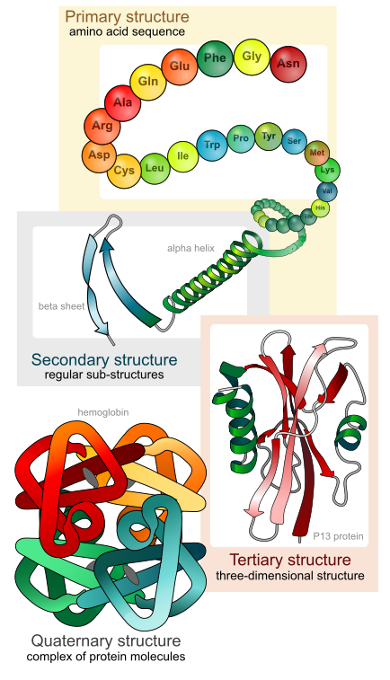
A fold (or topology) is the overall arrangement of secondary-structure elements. Two proteins with completely different sequences can share the same fold: different bricks, same floor plan. A domain is a compact, independently folding unit within a larger protein; many proteins consist of multiple linked domains.

Evolution and MSAs

Related proteins across species, called homologs, share a common ancestor. Lining up homologous sequences produces a multiple sequence alignment (MSA), which reveals conservation: positions that remain fixed across millions of years of evolution are usually structurally or functionally critical.

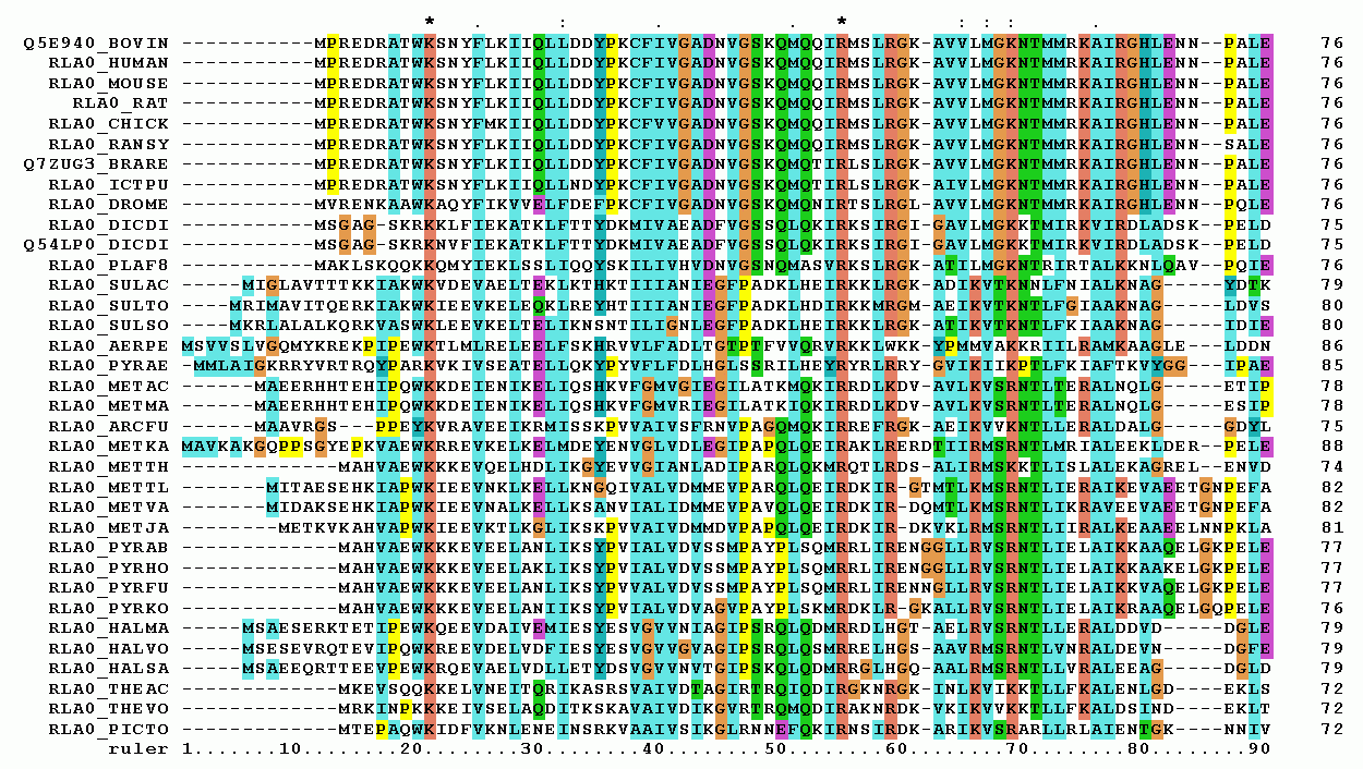
MSAs also reveal coevolution — positions whose substitutions are statistically coupled. Such couplings can provide evidence of structural contacts, although phylogeny and indirect correlations also contribute. This was the key insight behind early contact prediction methods and a core input to AlphaFold2. For ML researchers, MSAs are the protein equivalent of a large unlabeled dataset: they encode structural constraints without explicit 3D labels.

The organizing principle of structural biology is the sequence → structure → function triangle: sequence determines the 3D fold, and the fold determines what the protein does.

---

What Holds the Shape Together

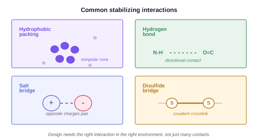
A protein folds because the folded state is thermodynamically favorable. The dominant driving force is the hydrophobic effect: nonpolar side chains are energetically penalized when exposed to water, so the chain collapses to bury them in a tightly packed interior, the hydrophobic core. Disrupting this core usually destroys the protein.

On top of the hydrophobic effect, several other forces contribute:

• Hydrogen bonds — weak electrostatic attractions between donor and acceptor atoms. Individually weak, but collectively essential for secondary structure. Every backbone N-H and C=O must either form an H-bond or be exposed to water; an unsatisfied H-bond donor buried in the core is energetically costly.
• Salt bridges — attractions between positively charged residues (Lys, Arg) and negatively charged ones (Asp, Glu). Contribute to stability on the protein surface.
• Disulfide bonds — covalent bonds between two cysteine residues. Molecular staples that physically lock distant parts of the chain together. Common in antibodies and secreted proteins.
• Van der Waals interactions — weak attractions between atoms at close range. Individually small, but they add up as thousands of atoms pack tightly in the core.

Stability and Failure Modes

Stability measures how hard it is to unfold a protein. The melting temperature (T\(_m\)) is the temperature at which half the protein population is unfolded — higher T\(_m\) means a more stable protein. A useful stability target depends on the application, storage conditions, and assay; there is no universal 60°C cutoff.²

The most common failure mode in protein design is aggregation: proteins stick to each other and form useless clumps, like egg whites cooking. This usually happens because hydrophobic patches that should be buried are instead exposed on the surface. Solubility — whether the protein stays dissolved in water — is closely related. An insoluble protein is useless regardless of how good it looks in simulation.

---

What Proteins Do — Binding and Function

Most proteins function by binding to other molecules — other proteins, small molecules, DNA, or metal ions. The strength of binding is quantified by the dissociation constant K\(_d\):³ lower K\(_d\) means tighter binding (the two molecules are harder to pull apart).

K\(_d\) range	Binding strength	Typical context
< 1 nM	Very tight	Therapeutic antibodies
1–100 nM	Tight	Designed binders, drugs
100 nM – 1 μM	Moderate	Signaling interactions
> 1 μM	Weak	Transient contacts

Specificity is the other binding constraint: a binder that grabs everything is useless. The physical contact surface between two binding partners is the binding interface, typically spanning 1,000–2,000 Å\(^2\). Interface residues do not contribute equally; a handful of hotspot residues provide most of the binding energy. Identifying target-surface hotspots is the first step of binder design.

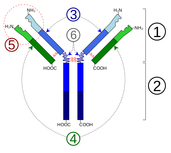
For antibodies specifically, the target surface is called the epitope and the matching surface on the antibody is the paratope. Different antibodies can target different epitopes on the same target protein.

Beyond binding, enzymes catalyze chemical reactions. Their active sites, small pockets with precisely positioned catalytic residues, accelerate reactions by factors of 10\(^6\)–10\(^{12}\). Enzyme design is harder than binder design because it requires exact 3D geometry, not merely a good surface fit.

Proteins can also undergo conformational changes — shifts in 3D structure triggered by binding. This is how signals propagate through biological systems: binding at one site rearranges the protein to expose or hide a distant functional site.

---

How Protein Designers Think

Protein designers turn structural knowledge into testable questions: Are hydrophobic residues buried? Are hydrogen-bond donors and acceptors satisfied? Is the backbone in a favorable region of Ramachandran space?⁴ These checks help explain a model’s failures, even when they are not sufficient to predict function.

Many of these heuristics translate naturally into energy-function terms, loss functions, and model inductive biases.

Energy Landscapes

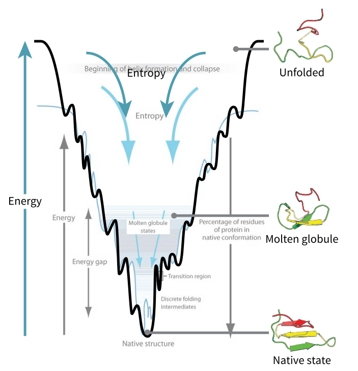
The folded state of a protein sits at the bottom of a free energy landscape, a surface over all possible conformations. Design means finding sequences whose energy minimum matches a target structure. It is an optimization problem.

Packing Geometry

When a designer says “the hydrophobic core is well-packed,” they mean atoms fill space tightly with no voids. This is quantified by packing density metrics and reflected in the van der Waals energy term in Rosetta. Empty space in the core means unfavorable energetics.

Hydrogen Bond Networks

“Satisfying all hydrogen bonds” has a precise meaning: every buried backbone or side-chain donor/acceptor must have a partner. An unsatisfied H-bond donor buried in the core costs roughly 5 kcal/mol, enough to destabilize the entire protein. Designers check these systematically.

Shape Complementarity

Binding interfaces are scored by geometric fit using the Sc score, which measures how well the two surfaces fit together (like interlocking fingers). Sc = 1.0 is a perfect fit; most natural protein–protein interfaces score 0.6–0.7. This is a geometric computation, not a subjective judgment.

Systematic Enumeration

Rosetta’s design protocol is Monte Carlo sampling over sequence space with a physics-based energy function. At each position, Rosetta tries different amino acid identities and side-chain rotamers,⁵ accepts or rejects changes based on the energy function, and iterates. The transition from Rosetta to ML-based design was not a complete change in goals; it replaced a physics-based MCMC optimizer with learned models.

Biologist Reasoning Is ML Reasoning

Three examples of “structural biology intuition” translated to ML terms:

What a biologist says	What they mean computationally
“This helix should be amphipathic (hydrophobic on one side, hydrophilic on the other)”	The hydrophobic moment vector should point inward — a periodic constraint on sequence hydrophobicity with period 3.6 (the helix repeat)
“The core isn’t packed well”	Atoms have too much empty space — packing density below threshold, Rosetta vdW energy too high
“How well defined is that loop?”	A high crystallographic B-factor can reflect motion or disorder; low pLDDT indicates prediction uncertainty. They are not interchangeable measures of flexibility.

The domain knowledge ML researchers admire in structural biologists is largely a set of quantitative constraints and heuristics that map to loss terms and architectural priors. When a biologist says something about a structure, there is usually a computable quantity behind it.

---

The Design Problem — Formulations and Types

Protein design decomposes into three ML problem formulations:

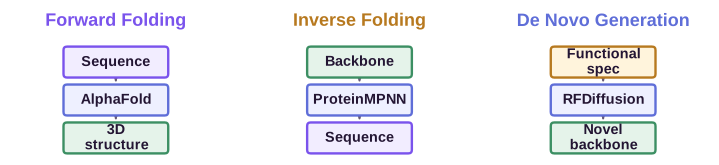
Forward folding (structure prediction). Input: amino acid sequence. Output: 3D atomic coordinates. Model: AlphaFold2. This is the “check your work” step: given a designed sequence, does the predicted fold match the intended structure?

Inverse folding (sequence design). Input: 3D backbone coordinates. Output: amino acid sequence that folds into that backbone. Model: ProteinMPNN. This is the core design step: “I drew the blueprint; now find the bricks.”

De novo backbone generation. Input: functional specification (target protein, hotspot residues, symmetry constraints). Output: new backbone structure. Model: RFDiffusion. This is the generative step: “create a new shape that binds this target.”

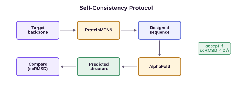
The standard validation loop ties these together: generate a backbone (RFDiffusion) → design a sequence for it (ProteinMPNN) → predict the structure of that sequence (AlphaFold) → compare the prediction to the intended backbone. If they match, the design is self-consistent.

What People Design

Design targets:

• Miniproteins (40–80 residues) — small, stable, easy to produce. The “Hello World” of protein design.
• De novo binders — proteins that grab a specific target surface. The most active area in computational design.
• Antibodies — Y-shaped immune proteins. Design focuses on the six CDR loops (especially CDR-H3), which contact the antigen. The stable framework regions hold the CDRs in position.
• Nanobodies (VHH) — single-domain antibodies from camelids (camels, llamas). Smaller, simpler to engineer computationally.
• Peptides — short chains, often flexible. The size boundary between a peptide and a protein varies by convention; short sequence length does not imply a single stable fold.
• Enzymes — proteins that catalyze chemical reactions. Harder than binder design: requires precise 3D geometry at the active site.
• Vaccine immunogens — engineered proteins that train the immune system. The COVID-19 spike protein vaccines are a high-profile example.

Design Constraints

Real designs are constrained:

• Hotspot residues — “the designed binder must contact these specific residues on the target.”
• Motif scaffolding — “build a stable protein around this functional fragment, holding it in the correct 3D position.”
• Symmetric design — “generate identical subunits that assemble into a ring, cage, or icosahedron (a 20-faced sphere-like shell).”
• Contig notation — RFdiffusion’s input format. For example, A1-100/0 30-50 retains residues 1–100 of the input chain A and designs a separate 30–50-residue chain. The /0 marks a chain break; its following space is significant. See the official examples (RFdiffusion documentation).

---

The Computational Toolkit

Seven tools define the current protein design stack. For each, the key questions are what goes in, what comes out, and when to use it.

Rosetta

Rosetta is the classic physics-based suite, developed over more than 20 years (Leman et al., 2020). It evaluates designs with an energy function that sums van der Waals packing, electrostatics, hydrogen bonds, solvation, and backbone geometry terms. Output is reported in Rosetta Energy Units (REU), where lower is better. Rosetta is still widely used for scoring and refinement, even as ML tools handle generation.

AlphaFold2 / AlphaFold3

Input: sequence (+ MSA for AF2). Output: predicted 3D structure with per-residue and per-pair confidence scores.

• pLDDT — per-residue confidence (0–100). High pLDDT means the model is certain about local structure.
• pTM — overall fold confidence.
• ipTM — interface confidence for protein complexes. The key metric for binder design.
• PAE — predicted aligned error matrix. Shows expected positional error between all residue pairs. For binder design, check the inter-chain PAE block: low values mean the model is confident about the binding mode.

AF2 handles single chains (Jumper et al., 2021); AF2-Multimer extends it to multi-chain protein complexes. AF3 extends to protein–nucleic acid and protein–small molecule complexes (Abramson et al., 2024).

ESMFold

ESMFold predicts structure from a single sequence without constructing an MSA (Lin et al., 2023). This makes it useful for a first computational screen of a large sequence pool. A faster predictor changes screening cost, but its disagreements and biases must still be checked before choosing which candidates to test.

ProteinMPNN

Input: 3D backbone coordinates (as a graph of residue positions). Output: amino acid probability distribution at each position. A message-passing neural network that designs sequences for given backbones (Dauparas et al., 2022). Fast, accurate, and the standard inverse folding tool. Typically generates 8–16 sequences per backbone.

RFDiffusion

Input: target protein structure + conditioning constraints (hotspot residues, motifs, symmetry). Output: new backbone coordinates. A denoising diffusion model over backbone coordinates — analogous to image diffusion models but operating in SE(3) coordinate space. RFDiffusion is a standard tool for de novo backbone generation (Watson et al., 2023).

Boltz / Boltz2

Boltz models are alternative structure predictors that provide a second opinion on AlphaFold (Wohlwend et al., 2024). Agreement between two separately trained predictors is not experimental proof, but it is a useful computational sanity check before spending lab effort.

BoltzGen

BoltzGen (Stark et al., 2025) is worth one sentence here because it keeps the same design loop but couples the steps more tightly. The core workflow is still generate, sequence, predict, filter, and validate. Newer systems mostly change how tightly those steps interact and which failure modes they catch before experiments.

What Does “Good” Look Like?

A reference table for interpreting computational metrics:

Metric	Example interpretation	Limitation
pLDDT	A filter such as > 80 selects locally confident predictions	Confidence, not measured stability
ipTM	A filter such as > 0.8 selects confident complex arrangements	Not a binding-affinity measurement
scRMSD	< 2 Å is one possible backbone-agreement filter	Model self-consistency, not experimental validation
K\(_d\)	< 100 nM indicates tight binding in many assay settings	Experimental conditions and application determine the useful range
Rosetta energy	Compare designs scored under the same protocol	No universal zero threshold; size and composition affect the score

These example cutoffs are not a universal acceptance recipe. Calibrate filters against experiments for the target and model versions being used.

---

The Design Workflow

The tools above assemble into a five-step pipeline. To make the bookkeeping concrete, consider the illustrative counts below. They are chosen to explain the workflow and are not experimental results or expected hit rates.

Step 1: Define the problem

What should the protein do? Bind a specific target surface? Catalyze a reaction? Form a symmetric cage? This determines which tools to use, which constraints to set, and how to evaluate success. For binder design, you identify the target protein, choose an epitope (the surface patch to target), and specify hotspot residues.

Step 2: Generate backbones

RFDiffusion generates ~10,000 backbone structures conditioned on the target and constraints. Each backbone is a candidate protein shape: no sequence yet, just the 3D arrangement of backbone atoms.

Step 3: Design sequences

In this example, ProteinMPNN generates eight sequences per backbone: 80,000 candidate sequences in total. Each is conditioned on its target backbone.

Step 4: Computational filtering

The self-consistency check eliminates most candidates. For each designed sequence:

1. Predict its structure with AlphaFold or ESMFold.
2. Compare the predicted structure to the intended backbone (scRMSD).
3. Check confidence metrics (pLDDT, ipTM for binders).

Suppose 1% pass the chosen filters: 800 of the 80,000 sequences remain. This assumed rate is only part of the illustrative bookkeeping.

Step 5: Experimental validation

The top ~20 candidates are ordered as synthetic genes and tested in the lab:

• Expression — bacteria (usually E. coli) produce the designed protein from synthetic DNA. Many designs fail here: the protein doesn’t express or is insoluble.
• Purification — the protein is isolated from the bacterial cell contents. For a soluble-binder campaign, aggregation or insolubility complicates purification and may rule out a candidate.
• CD (circular dichroism) — a quick test for secondary structure. The spectrum tests whether the observed secondary structure is consistent with the design; it does not determine the full fold.
• SPR (surface plasmon resonance) — measures binding affinity in real time, providing the K\(_d\) value. It is one assay of affinity and kinetics, not a complete measure of binder quality.
• Display methods (phage display, yeast display) — screen millions of variants simultaneously. Each variant is displayed on the surface of a phage or yeast cell, washed over the target, and only binders stick. Used to improve initial hits.
• Directed evolution — the pre-ML baseline. Randomly mutate, test, keep the best, repeat. Won the 2018 Nobel Prize in Chemistry. Computationally, this is what evolutionary algorithms replicate.
• Cryo-EM / X-ray crystallography — determine the actual 3D atomic structure. The definitive validation: did the protein fold into the intended shape? Slow and expensive, reserved for the most promising candidates.

An illustrative outcome might be 10 soluble proteins and 3–5 binders among 20 tested designs. Actual rates can differ substantially; report the target, assay, selection procedure, and number tested whenever giving an experimental hit rate.

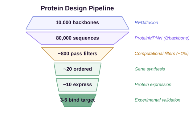
The practical question is how many useful proteins a fixed experimental budget recovers. Increasing a computational pass rate alone can simply admit more false positives. Evaluate filters prospectively, measuring expression and binding among selected candidates as well as how many distinct designs they retain.

---

References

• RosettaCommons. RFdiffusion: contig mapping and motif scaffolding. Official documentation. ↩

• Cao, L., et al. (2020). De novo design of picomolar SARS-CoV-2 miniprotein inhibitors. Science, 370(6515), 426-431. DOI. ↩
• Hsieh, C.-L., et al. (2020). Structure-based design of prefusion-stabilized SARS-CoV-2 spikes. Science, 369(6510), 1501-1505. DOI. ↩
• Leman, J. K., et al. (2020). Macromolecular modeling and design in Rosetta: recent methods and frameworks. Nature Methods, 17, 665-680. DOI. ↩
• Jumper, J., et al. (2021). Highly accurate protein structure prediction with AlphaFold. Nature, 596, 583-589. DOI. ↩
• Dauparas, J., et al. (2022). Robust deep learning-based protein sequence design using ProteinMPNN. Science, 378(6615), 49-56. DOI. ↩
• Lin, Z., et al. (2023). Evolutionary-scale prediction of atomic-level protein structure with a language model. Science, 379(6637), 1123-1130. DOI. ↩
• Watson, J. L., et al. (2023). De novo design of protein structure and function with RFdiffusion. Nature, 620, 1089-1100. DOI. ↩
• Abramson, J., et al. (2024). Accurate structure prediction of biomolecular interactions with AlphaFold 3. Nature, 630, 493-500. DOI. ↩
• Wohlwend, J., et al. (2024). Boltz-1: Democratizing Biomolecular Interaction Modeling. bioRxiv. ↩
• Stark, H., et al. (2025). BoltzGen: Toward Universal Binder Design. bioRxiv. ↩