Genomic Foundation Models and Virtual Cells

Adapted from my 2025 Machine Learning for Molecules and Geometric Deep Learning lectures. Sequence, measured cell state, and response to intervention are different modeling objects with different evidence requirements; the central question is which of them destructive genomic and single-cell measurements can actually identify.

Calling DNA a language is productive, but incomplete. A genomic sequence has local motifs, long-range dependencies, repeated elements, and variation across organisms. These regularities make masked or autoregressive pretraining useful. Yet a cell is not the text of its genome. Cells with essentially the same DNA can occupy different states because transcription factors, chromatin, proteins, metabolites, spatial signals, developmental history, and environment differ.

The same distinction appears one level later. A single-cell RNA-sequencing vector is not a cell state in full; it is a sparse, destructive measurement of part of that state. And a model that reconstructs or embeds those measurements is not automatically a simulator of intervention. Predicting what happens after a drug, gene edit, or cytokine requires conditional data, temporal assumptions, and evaluation on interventions and contexts absent from training.

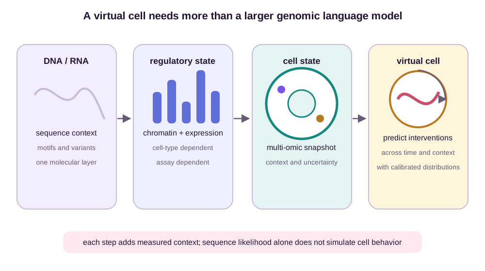
The phrase virtual cell should therefore be reserved for a stronger claim: a model that predicts distributions over future cellular behavior under specified interventions and contexts, exposes its uncertainty, and remains useful when some combination of donor, cell type, environment, perturbation, or time was not observed during training.

One hypothetical program will make that claim testable. Consider a regulatory variant upstream of a cytokine receptor. We will follow its evidence through four genes—\(\mathrm{JAK1}\), \(\mathrm{STAT1}\), \(\mathrm{IRF1}\), and the negative-feedback regulator \(\mathrm{SOCS1}\)—after cytokine exposure. The sequence model scores the variant; regulatory assays attach a context-specific label; counts observe four noisy molecular outputs; a latent state compresses them; a perturbation model predicts responder and nonresponder populations; and a donor-level experiment decides whether the prediction transfers. Each interface changes the random variable. None permits a stronger claim merely because the same embedding appears on both sides.

DNA language models compress sequence distributions

Let a DNA segment be

\[\mathbf s=(s_1,\ldots,s_L), \qquad s_i\in\{\mathrm A,\mathrm C,\mathrm G,\mathrm T\}.\]

A masked genomic model selects positions \(M\) and minimizes

\[\mathcal L_{\mathrm{mask}} = -\sum_{i\in M} \log p_{\theta} \!\left(s_i\mid\widetilde{\mathbf s}\right).\]

Early models such as DNABERT tokenized overlapping \(k\)-mers and showed that pretraining on a reference genome could transfer to promoter, splice-site, and transcription-factor-binding tasks (Ji et al., 2021). Modern models use single nucleotides or learned tokens, longer context, more species, and architectures whose cost grows more gently with sequence length.

Tokenization changes the inductive bias. Overlapping \(k\)-mers expose motifs but create leakage within a naive masking task: neighboring tokens share most of their nucleotides. Single-base tokens remove that shortcut but demand longer effective context. Learned tokens compress recurring substrings, yet their boundaries need not coincide with regulatory elements.

For a finite example, tokenize \(\mathrm{ACGTAC}\) into overlapping 3-mers:

\[(\mathrm{ACG},\mathrm{CGT},\mathrm{GTA},\mathrm{TAC}).\]

Masking only \(\mathrm{CGT}\) does not hide its bases. The left token reveals \(\mathrm{CG}\) and the right token reveals \(\mathrm{GT}\), so their overlap reconstructs all three characters. More generally, an interior nucleotide appears in \(k\) adjacent \(k\)-mers. If tokens are masked independently with probability \(m=0.15\), the probability that every token containing that nucleotide is hidden is \(m^k\). For 6-mers this is \(0.15^6\approx1.14\times10^{-5}\), even though 15% of tokens were nominally masked. Span masking or single-base tokenization changes the task from overlap completion back toward sequence inference.

DNA is double-stranded, so strand handling must also match the task. If a label is invariant to reverse complementation, the predictor should satisfy

\[f_{\theta}(\mathbf s) = f_{\theta}(\operatorname{RC}(\mathbf s)),\]

or be trained so the two orientations agree. Directional tasks such as transcription relative to a promoter are different: reversing the sequence also changes the coordinate system and output orientation. “Reverse-complement invariance” cannot be applied indiscriminately.

The semantics are visible on five bases. For \(\mathbf{s}=\mathrm{ACGTT}\), the reverse complement is \(\operatorname{RC}(\mathbf{s})=\mathrm{AACGT}\). An orientation-free enhancer-activity label should assign both sequences the same scalar. A directional transcription profile is different. If the plus-oriented target across the five positions is \((0,1,4,2,0)\), then reversing coordinates gives \((0,2,4,1,0)\) and swaps the strand label. Averaging the two vectors would create \((0,1.5,4,1.5,0)\), a target belonging to neither orientation. Invariance is correct for the first task; equivariant reversal of the output is correct for the second.

Sequence likelihood is already useful for variant scoring:

\[\Delta_{\mathrm{LM}} = \log p_{\theta}(s_i=s_i^{\mathrm{alt}}\mid\mathbf s_{\setminus i}) - \log p_{\theta}(s_i=s_i^{\mathrm{ref}}\mid\mathbf s_{\setminus i}).\]

This measures compatibility with the learned sequence distribution. It is not a causal effect on expression, phenotype, or disease. Conservation, mutational processes, genomic repeats, and sampling across species all contribute to likelihood.

Regulatory genomics needs labels beyond sequence

Promoters, enhancers, splice sites, and transcription-factor motifs are sequence-defined in part, but their activity depends on cellular context. A long sequence model can predict tracks such as chromatin accessibility, protein binding, or RNA abundance:

\[f_{\theta}(\mathbf s) = \widehat{\mathbf y} \in\mathbb R^{B\times K},\]

where \(B\) indexes genomic bins and \(K\) indexes assays, tissues, or cell types. Enformer combined convolutional feature extraction with attention over a roughly 200-kilobase input and predicted thousands of functional genomic tracks, demonstrating the value of distal context for expression and variant-effect prediction (Avsec et al., 2021).

This is supervised multitask learning, not merely genomic language modeling. The targets anchor the representation to measured regulatory function. They also import assay noise, uneven cell-type coverage, and batch structure. A model can predict an ATAC-seq track accurately because similar genomic loci or cell types were seen during training; that result does not by itself show transfer to a new donor or regulatory program.

Long context is a capacity, not proof that distal regulation has been learned. Models may rely primarily on promoter-proximal motifs even when given a megabase. Evaluation should stratify variants and regulatory elements by distance, test experimentally perturbed enhancers, and compare against local-context ablations.

Return to the cytokine-response variant. Suppose the sequence model assigns the alternative allele a favorable log-likelihood ratio, while a lymphocyte ATAC-seq head predicts a twofold accessibility increase in the receptor enhancer. The first number concerns compatibility with the training sequence distribution. The second is a supervised prediction for a named assay and cell context. Neither yet establishes that editing the allele changes \(\mathrm{JAK1}\)–\(\mathrm{STAT1}\) signaling: that causal step needs an allele-specific or edited regulatory experiment. Passing one embedding through both heads does not merge their evidentiary contracts.

RNA adds structure, processing, and abundance

RNA occupies several roles at once. Its primary sequence determines base-pairing possibilities and protein-binding motifs. Pre-mRNA is spliced into isoforms. Messenger abundance is a context-dependent output of regulation and degradation. Treating every RNA problem as next-token prediction hides these distinctions.

For splicing, a model may predict a distribution over donor and acceptor choices conditional on genomic sequence. For RNA structure, the output may be a base-pairing matrix or three-dimensional conformation. For transcript abundance, sequence is insufficient without cell context. A variant that alters one splice site can have different consequences across tissues because the relevant RNA-binding proteins differ.

The useful representation therefore follows the claimed output: nucleotide embeddings for local motifs, pair representations for base pairing, long genomic context for isoform regulation, and cellular covariates for expression. A single “RNA embedding” is not a universal object.

Our regulatory variant need not alter any transcript sequence. It may change receptor abundance and thereby shift downstream \(\mathrm{STAT1}\) and \(\mathrm{IRF1}\) RNA counts only after cytokine exposure. An RNA sequence encoder can still represent splice or stability determinants of those transcripts, but it lacks the intervention and donor state that activates the program. The same four gene names therefore denote different objects across interfaces: nucleotide strings in an RNA model, latent abundances in a cell model, and noisy counts in an assay.

A single-cell matrix is an observation model

For cell \(c\) and gene \(g\), RNA sequencing returns an integer count \(Y_{cg}\). A useful abstraction is

\[Y_{cg} \sim \operatorname{NB} \!\left(\mu_{cg}=\ell_c\lambda_{cg},\phi_g\right),\]

where \(\lambda_{cg}\) is latent relative abundance, \(\ell_c\) is library size or capture efficiency, and \(\phi_g\) controls overdispersion. Deep generative models such as scVI explicitly use a probabilistic count model while separating biological latent variables from technical covariates (Lopez et al., 2018).

Use the negative-binomial parameterization

\[\operatorname{Var}(Y_{cg}) =\mu_{cg}+\frac{\mu_{cg}^2}{\phi_g}, \qquad P(Y_{cg}=0) =\left(\frac{\phi_g}{\phi_g+\mu_{cg}}\right)^{\phi_g}.\]

For a transcript with relative abundance \(\lambda=0.02\) and dispersion \(\phi=2\), a cell with library factor \(\ell=100\) has \(\mu=2\), variance \(4\), and zero probability \((2/4)^2=0.25\). At \(\ell=1000\), the same relative abundance gives \(\mu=20\), variance \(220\), and zero probability \((2/22)^2\approx0.0083\). A zero is therefore about 30 times more likely in the shallower library without any change in underlying abundance.

For the running program, a baseline cell might yield four-gene counts \((2,0,1,3)\) for \((\mathrm{JAK1},\mathrm{STAT1},\mathrm{IRF1},\mathrm{SOCS1})\). Those integers are observations, not the latent molecular state. A second draw from the same state can differ, and a tenfold deeper library changes their expected scale. The observation model is the interface that prevents count reconstruction error from being mistaken for biological-state error.

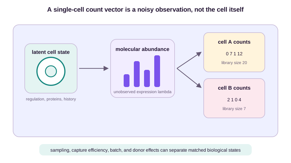
A zero can mean no transcript was present, the transcript was not captured, or sequencing depth was insufficient. Conversely, a large count can partly reflect a large library. Normalization and log transformation stabilize learning but change the statistical object. Ranking genes, as some cell language models do, removes absolute scale and emphasizes relative expression.

That loss is exact for abundance vectors \((100,40,10,1)\) and \((10,4,1,0.1)\). Both rank the four genes in the same order, so a rank-only encoder receives the same token sequence. Yet every abundance differs by a factor of ten. Rank is useful when library scale is nuisance; it is unsafe when total program amplitude distinguishes a weak cytokine response from a strong one. The protein representation chapter develops the same general lesson from another domain: information can be present in the original object yet inaccessible after a chosen encoding.

The analogy between a cell and a sentence is therefore limited. Genes have a fixed identity rather than a natural word order. Expression is quantitative, and multiple genes can be active simultaneously. A token sequence produced by sorting genes is an encoding choice, not biological chronology.

Cell foundation models learn reusable state encoders

Large cell models pretrain on millions of transcriptomes using masked genes, ranked expression sequences, binned values, or count-aware objectives. Geneformer trained a rank-based Transformer over single-cell transcriptomes and transferred it to network-biology tasks (Theodoris et al., 2023). scGPT jointly represents gene identities and expression values and applies generative pretraining across single-cell and multi-omic tasks (Cui et al., 2024).

Scaling helps when the corpus adds biological coverage: more donors, tissues, diseases, developmental stages, species, and measurement technologies. Merely adding more cells from a dominant cell line reduces optimization noise without expanding the support of the problem. Dataset size should therefore be reported alongside the number and balance of donors, studies, tissues, cell types, and conditions.

There is also no neutral cell embedding. An objective that reconstructs highly expressed genes may prioritize housekeeping programs. Batch integration can deliberately erase study identity but also erase a biological effect confounded with study. Cell-type classification encourages stable identity while a perturbation task needs sensitivity to transient response.

Suppose an encoder maps the normalized four-gene baseline \((2,0,1,3)\) to latent coordinates \(z=(0.2,0.7)\), interpreted by a downstream probe as pathway activation and negative feedback. After cytokine, counts such as \((8,12,20,5)\) map to \((2.1,0.9)\). The coordinates are learned summaries, not measured biochemical concentrations. Their usefulness must be established by decoding held-out response, transfer to new donors, and stability to library-size changes. A batch classifier failing to decode \(z\) only shows that one classifier cannot recover batch; it does not prove that the latent state contains biology alone.

Multimodal embeddings align partial views of state

Single-cell assays can measure RNA, chromatin accessibility, surface proteins, methylation, spatial location, morphology, or imaging phenotypes. Let \(x_c^{(m)}\) be modality \(m\) for cell \(c\). A multimodal encoder produces

\[z_c^{(m)}=f_m\!\left(x_c^{(m)}\right)\]

and may align paired modalities using a contrastive loss:

\[\mathcal L_c = -\log \frac{\exp(\operatorname{sim}(z_c^{(r)},z_c^{(a)})/\tau)} {\sum_{c'}\exp(\operatorname{sim}(z_c^{(r)},z_{c'}^{(a)})/\tau)},\]

where \(r\) and \(a\) might denote RNA and ATAC. Alignment is useful for annotation transfer and missing-modality prediction. It does not make RNA and chromatin interchangeable. Their shared latent state may omit modality-specific variation needed for a downstream mechanism.

A three-cell batch shows what the contrastive denominator declares. Let the RNA-to-ATAC similarities, with temperature \(\tau=1\), be

\[\mathbf S= \begin{pmatrix} 4&1&0\\ 1&3&2\\ 0&2&3 \end{pmatrix},\]

where the diagonal entries are paired measurements. Cell 1 receives positive probability

\[\frac{e^4}{e^4+e^1+e^0}\approx0.936, \qquad \mathcal L_1\approx0.066.\]

For cell 2 the positive probability is \(e^3/(e^1+e^3+e^2)\approx0.665\) and \(\mathcal L_2\approx0.408\). If cells 2 and 3 are two cytokine responders in the same biological state, their similarity \(S_{23}=2\) is treated as a negative solely because they are different rows. The loss learns paired-cell identity and batch composition as well as shared biology. A donor-aware batch or multi-positive objective changes that invariance claim; scaling the encoder does not.

Spatial context adds another layer. A cell’s neighbors, tissue compartment, extracellular signals, and geometry can affect its response. Treating cells as independent tokens discards this coupling. A virtual cell intended for tissue biology eventually needs an interaction model, not only a better isolated-cell embedding.

Perturbation models predict transitions, not labels

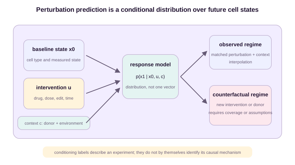
Let \(x_0\) be a baseline cell state, \(u\) an intervention, \(c\) context, and \(t\) elapsed time. The target is a conditional distribution

\[p_{\theta}(x_t\mid x_0,u,c,t),\]

not just one mean expression vector. The intervention may be a gene knockout, CRISPR activation, drug structure, dose, cytokine, combination, or environmental change.

A simple latent composition assumes

\[z_t = z_{\mathrm{basal}}(x_0) +e_u(u) +e_c(c) +e_t(t),\]

followed by a decoder to expression. CPA uses this compositional idea to combine basal state, perturbation, dosage, and covariates, enabling predictions for held-out combinations (Lotfollahi et al., 2023). The factorization is interpretable and data-efficient, but additivity is an assumption. Drug synergy, gene epistasis, saturation, and state-dependent response require interaction terms or richer dynamics.

Predicting the mean response can also erase biologically meaningful heterogeneity. A treatment may split cells into responding and resistant subpopulations. Two models with identical mean-squared error can differ sharply: one produces both modes, while the other predicts an implausible average cell between them.

In the cytokine experiment, suppose 50 cells remain near \((2,1,1,3)\) and 50 enter a responder state \((10,15,21,3)\). The population mean is \((6,8,11,3)\). No cell has that profile. Under squared error the conditional mean is the optimal point prediction, so good mean-squared error can reward a state lying midway between resistance and response. A distributional model must instead recover two modes with approximately 0.5 mass each and report how that mixture changes across donor, dose, and time.

Conditioning is not causal identification

Experimental perturbation gives stronger evidence than observational correlation, but a learned conditional distribution is not automatically a causal model. The desired object is closer to

\[p\!\left(x_t\mid\operatorname{do}(u),x_0,c\right),\]

where \(\operatorname{do}(u)\) denotes an intervention. Identification still depends on experimental design. Cells assigned different treatments may come from different batches. Viability selection changes which cells remain measurable. Baseline state is often observed in control cells rather than the exact cells later destroyed for sequencing. Dose and time may be confounded.

Destructive snapshots identify population marginals, not cell trajectories. Collapse the latent state to low response \(L\) or high response \(H\). Suppose both baseline and six-hour samples contain half \(L\) and half \(H\). With row vectors for population probabilities, two row-stochastic transition matrices fit those marginals:

\[\mathbf T_{\mathrm{stay}} = \begin{pmatrix}1&0\\0&1\end{pmatrix}, \qquad \mathbf T_{\mathrm{swap}} = \begin{pmatrix}0&1\\1&0\end{pmatrix}.\]

For \(\boldsymbol\pi_0=(0.5,0.5)\), both give \(\boldsymbol\pi_0\mathbf T=(0.5,0.5)\). The first says every cell retains its state; the second says every cell switches. Their endpoint marginals are identical, while their individual counterfactual responses are opposite. The distinction between a transition kernel and its induced marginal mirrors the path-versus-density distinction, but here the kernel is not supplied by a physical SDE. Lineage barcodes, live-cell reporters, nondestructive longitudinal measurements, or a justified structural transition model are needed to choose between these couplings.

Gene deletion by masking a token in a pretrained transcriptome model is especially easy to overinterpret. Removing a gene from the input asks how the encoder changes under missing information. A biological knockout changes transcription, protein abundance, feedback, growth, and selection over time. Without perturbation data or a defensible mechanistic model, the two operations are not equivalent.

Causal claims should therefore follow the data. Randomized interventions can support response prediction within covered contexts. Compositional generalization requires held-out combinations. Mechanism discovery needs additional evidence: replicated interventions, temporal measurements, mediators, orthogonal assays, and prospective validation.

Batch, donor, and cell-line signals are predictive shortcuts

Single-cell corpora merge studies generated with different platforms, protocols, laboratories, reference genomes, and quality filters. Biological composition also varies across studies. If every disease sample was processed in one batch and every control in another, removing batch is statistically inseparable from removing disease without additional design.

The same failure can manufacture a cytokine effect. Suppose the observed mean \(\mathrm{IRF1}\) counts are

Batch	Control	Cytokine
A	4 from 100 cells	not measured
B	not measured	12 from 100 cells

In the additive model \(E[Y]=\alpha+\beta u+\gamma\mathbf 1\{\text{batch B}\}\), the table identifies only \(\beta+\gamma=8\). A pure treatment effect \((\beta,\gamma)=(8,0)\) and a mostly technical shift \((2,6)\) fit equally well. No representation can separate them from these observations. Measuring control and cytokine in both batches, with randomized allocation and biological replication, makes the two coefficients estimable.

Three confounders deserve special attention:

• Donor: genetic background, age, sex, treatment history, and environment can dominate subtle perturbation effects.
• Cell line: immortalized lines carry stable genomic abnormalities and laboratory adaptation; success across wells is not transfer to primary cells.
• Batch: library chemistry, sequencing depth, operator, plate, and processing date can be decoded from embeddings and may correlate with labels.

Adversarial removal of these signals does not prove biological invariance. A safer evaluation groups entire donors, cell lines, plates, and studies, then reports both biological preservation and technical mixing. Metadata must be treated as part of the dataset, not an optional appendix.

Foundation-model scaling does not define a virtual cell

More parameters, longer context, and broader pretraining can improve loss and transfer. They do not determine whether a model answers an interventional question. A large masked-cell model may be an excellent encoder and a poor response simulator. A smaller perturbation-specific model may generalize better because its training data match the intervention.

The relevant scaling axes are not only parameter count:

• diversity and balance of donors, tissues, species, and disease states;
• number and chemical or genetic diversity of perturbations;
• dose, time, combination, and environmental coverage;
• paired modalities and spatial or temporal resolution;
• reproducibility across laboratories and platforms;
• quality of negative controls and intervention assignment.

A million near-replicate cells do not provide a million independent contexts. Effective sample size depends on the unit of generalization.

Consider eight donors with 5,000 cells each. The matrix has 40,000 rows. An 80:20 random cell split places roughly 4,000 training and 1,000 test cells from every donor on both sides, so the test set contains zero new donors. A donor split with six training donors and two test donors has 30,000 and 10,000 cells, but only two independent test units for donor transfer. Within-donor cells sharpen each donor’s response estimate; they do not turn two donors into 10,000 genetic and environmental backgrounds. If cell-level intraclass correlation is \(\rho=0.05\), the usual cluster design effect for 5,000 cells is \(1+(5000-1)\rho=250.95\). Even the cell-equivalent effective size is only \(40{,}000/250.95\approx159\), and donor-level uncertainty must still be estimated from eight donors.

Evaluation must match the claim

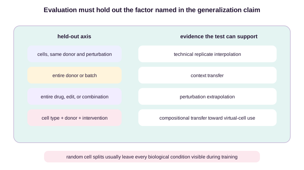
A random cell split is appropriate for denoising within an experiment. It is weak evidence for biological generalization because sibling cells from the same donor, batch, cell type, and perturbation appear on both sides.

Claim-matched evaluation should hold out the named axis:

Claim	Required holdout	Useful outputs
new cells in a known condition	individual cells	count likelihood, calibration
new donor or batch	entire donor/study	cell-type-stratified response
new perturbation	entire drug/edit	differential expression and distribution shift
new combination	all occurrences of that combination	synergy and interaction error
new cell type under treatment	cell type × intervention block	context-specific response
prospective virtual-cell use	future experiment/lab	calibrated predictions and failure detection

Metrics should also match the output. For average response, compare pseudobulk changes

\[\Delta_g = \mathbb E[X_g\mid u] - \mathbb E[X_g\mid u=0]\]

across genes, not only raw expression dominated by housekeeping genes. Report direction and magnitude on differentially expressed genes, but avoid selecting those genes on the test labels and then treating the subset as fixed. For distributions, use held-out likelihood when calibrated, energy distance or kernel discrepancies, cell-state proportions, and coverage of predictive intervals. For trajectories, test multiple times and recovery after intervention.

Strong baselines are essential. The control mean, nearest observed perturbation, additive single-perturbation model, cell-type average response, and linear dose model often capture much of a benchmark. A foundation model should beat the baseline that corresponds to its claimed novelty.

For a held-out donor in the running experiment, suppose the observed pseudobulk \(\mathrm{IRF1}\) increase is eight counts. Carrying the donor’s control mean forward predicts zero and has absolute error eight. The mean cytokine response among training donors predicts six and has error two. An additive model using the donor’s baseline predicts seven and has error one. A virtual-cell model predicting \(7.5\) has error \(0.5\). Comparing only with carry-forward would credit the model for learning an average cytokine effect; the donor-transfer claim is supported only by its improvement over the population and donor-conditioned baselines.

Point error does not say whether uncertainty is usable. Let the model issue 90% predictive intervals for pseudobulk response in 20 held-out donor–program blocks. If 18 intervals cover the observations, pooled empirical coverage is 90%. Suppose, however, that all 16 blocks from previously represented donors are covered while only 2 of 4 genuinely new-donor blocks are covered. The same result is 100% coverage for familiar donors and 50% for donor transfer. Calibration must be reported on the deployment stratum and at the unit of the claim; thousands of cells inside each block do not create thousands of interval trials.

What would a virtual cell need to predict?

A useful virtual cell should support at least five operations:

1. Represent state: integrate sequence, regulatory, molecular, spatial, and environmental evidence with missing modalities and uncertainty.
2. Predict interventions: return calibrated distributions for genetic, chemical, and environmental perturbations across dose and time.
3. Model dynamics: distinguish immediate signaling, transcriptional response, adaptation, division, death, and long-term state transitions.
4. Transfer compositionally: combine new donors, cell types, perturbations, and environments while recognizing unsupported combinations.
5. Guide experiments: identify which measurement would most reduce uncertainty, then update after the result.

This vision, articulated as an agenda for AI virtual cells by Bunne and colleagues, is explicitly multimodal, multiscale, predictive, and queryable (Bunne et al., 2024). It is closer to a scientific model connected to an experimental loop than to one universal embedding.

The cytokine program turns those operations into one prospective decision. Give the model the regulatory allele, a baseline distribution from a new donor, the cytokine intervention, assay context, and six-hour horizon. Suppose it predicts responder fraction \(0.70\) with a 90% interval \((0.48,0.84)\), compared with baseline fraction \(0.12\) and interval \((0.05,0.22)\). If a prespecified experiment-prioritization rule requires the lower response bound to exceed \(0.40\), this donor advances to a cytokine-blockade assay. The output supports allocating an experiment. It does not support treating a patient, identifying an individual cell’s path, or claiming that the regulatory allele caused the response until the corresponding randomized and allele-aware evidence exists.

Mechanistic fidelity will remain uneven. Some interventions can be predicted statistically from dense screens. Rare state transitions, long-term adaptation, metabolism, morphology, and tissue interactions may require explicit biological structure and new measurements. The model should say which regime it knows.

The useful boundary

Genomic foundation models compress sequence and can support regulatory annotation, variant scoring, and design. Cell foundation models compress noisy molecular snapshots and can support annotation, integration, retrieval, and task adaptation. Perturbation models learn conditional state changes within the support of intervention data.

These are substantial capabilities. None alone is a virtual cell.

A defensible virtual-cell interface should name its probability object. Let \(\widehat q_0\) be an empirical baseline distribution from control cells rather than a falsely paired baseline cell. For regulatory allele \(v\), intervention \(u\), context \(c\), and time \(t\), the model may return

\[\widehat p_{\theta} \!\left(x_t \mid \widehat q_0,v,\operatorname{do}(u),c,t,\mathcal D\right),\]

where \(\mathcal D\) denotes the training evidence that supports the prediction. The output is a distribution over measured future states. It becomes an individual transition kernel only if paired or lineage-resolved data, or an explicit identifiable dynamical assumption, supplies the missing coupling. It becomes a causal response distribution only under an intervention design that separates treatment from batch, survival, and context. It transfers to a donor population only when donor-held-out calibration supports that population.

Interface output	Supported claim	Missing evidence for the next claim
Sequence log-likelihood ratio	Variant compatibility under the genomic corpus	Context-specific regulatory assay
Predicted accessibility or expression track	Regulatory label in a named cell context	Randomized allele or enhancer perturbation
Count-aware latent state	Compressed observation after accounting for library and batch model	Protein, morphology, spatial state, and encoding sufficiency
Perturbation-conditioned marginal	Population response at a named dose and time	Cell-level coupling, lineage, or longitudinal dynamics
Donor-calibrated predictive distribution	Prospective experiment ranking in the validated donor population	Independent experimental outcome and mechanism

The contract also includes abstention. The model should flag when the allele, donor ancestry, cell type, intervention mechanism, dose, or assay platform lies outside calibrated support. A wide interval is useful only if it widens on those cases and its coverage has been measured there. A narrow interval inherited from an in-distribution validation set is not evidence of certainty in a new biological regime.

The stronger object begins when the model treats a cell as a partially observed dynamical system, distinguishes association from intervention, predicts response distributions rather than plausible-looking averages, and is evaluated on the contexts named in its claim. Scaling remains valuable, but only when it expands biological and experimental support—not when model size substitutes for the missing experiment.

References

1. Ji, Y., Zhou, Z., Liu, H., & Davuluri, R. V. (2021). DNABERT: Pre-trained Bidirectional Encoder Representations from Transformers Model for DNA-Language in Genome. Bioinformatics. ↩
2. Avsec, Ž. et al. (2021). Effective Gene Expression Prediction from Sequence by Integrating Long-Range Interactions. Nature Methods. ↩
3. Lopez, R., Regier, J., Cole, M. B., Jordan, M. I., & Yosef, N. (2018). Deep Generative Modeling for Single-Cell Transcriptomics. Nature Methods. ↩
4. Theodoris, C. V. et al. (2023). Transfer Learning Enables Predictions in Network Biology. Nature. ↩
5. Cui, H. et al. (2024). scGPT: Toward Building a Foundation Model for Single-Cell Multi-Omics Using Generative AI. Nature Methods. ↩
6. Lotfollahi, M. et al. (2023). Predicting Cellular Responses to Complex Perturbations in High-Throughput Screens. Molecular Systems Biology. ↩
7. Bunne, C. et al. (2024). How to Build the Virtual Cell with Artificial Intelligence: Priorities and Opportunities. Cell. ↩

---

Figure provenance. All four virtcell_ diagrams are original SVG illustrations generated by scripts/generate_virtcell_figures.py. They synthesize standard genomics, single-cell observation, perturbation-modeling, and evaluation concepts described in the cited primary literature; no third-party artwork is reproduced.