Geometric Flow Matching on Manifolds

Adapted from my 2025 Machine Learning for Molecules and Geometric Deep Learning lectures. This article identifies the geometric replacements that make ordinary flow matching valid on rotations, periodic angles, and other curved state spaces, then follows one state through loss, density change, symmetry, and numerical integration.

Flow matching is unusually easy to describe in Euclidean space. Sample noise \(x_0\) and data \(x_1\), connect them by a straight line, and train a velocity field to follow that line. The construction depends on operations so familiar that they become invisible: subtracting two points, adding a vector to a point, and measuring a squared error with one global inner product.

None of those operations is globally available on a general manifold. Two rotations cannot be averaged entry by entry and still remain rotations. The difference between two angles must respect periodicity. A velocity attached to one point on a sphere does not automatically live in the tangent space of another point.

Riemannian flow matching preserves the logic of flow matching while replacing its hidden Euclidean assumptions. Velocities live in tangent spaces. The exponential and logarithmic maps replace addition and subtraction. Geodesics replace straight lines. The Riemannian metric measures velocity error, and Riemannian divergence describes how the flow transports density. This is a small conceptual change with large consequences for molecular and geometric generation.

Euclidean flow matching learns a velocity field

The Euclidean construction below is only a reference interface. The preceding chapter derives why conditional regression recovers the marginal field and distinguishes that population identity from finite training. Here we ask a different question: which operations in that interface cease to be well-typed when the state is curved?

Let \(p_0\) be a tractable base distribution on \(\mathbb{R}^d\) and \(p_1\) the data distribution. A time-dependent vector field \(u_t:\mathbb{R}^d\to\mathbb{R}^d\) defines the ODE

\[\frac{d x_t}{dt}=u_t(x_t), \qquad x_0\sim p_0.\]

Its flow map \(\psi_t\) pushes the base distribution forward to a probability path \(p_t=(\psi_t)_\#p_0\). At the density level, the same evolution satisfies the continuity equation

\[\partial_t p_t(x) + \nabla\cdot\left(p_t(x)u_t(x)\right) =0.\]

Directly constructing the marginal velocity \(u_t\) is usually difficult. Flow matching instead chooses tractable conditional paths. For independently sampled endpoints \(x_0\sim p_0\) and \(x_1\sim p_1\), the simplest path is

\[x_t=(1-t)x_0+t x_1, \qquad u_t(x_t\mid x_0,x_1)=x_1-x_0.\]

Equivalently, when the current point and endpoint are known,

\[u_t(x_t\mid x_1)=\frac{x_1-x_t}{1-t}.\]

A neural field \(v_\theta(t,x)\) is trained with the conditional flow-matching objective

\[\mathcal{L}_{\mathrm{CFM}}(\theta) = \mathbb{E} \left[ \left\lVert v_\theta(t,x_t) -u_t(x_t\mid x_0,x_1) \right\rVert^2 \right].\]

Although the target depends on a particular endpoint pair, averaging these targets at a fixed \(x_t\) recovers the marginal velocity needed to transport the marginal path. This conditional-to-marginal identity is the central simplification of flow matching (Lipman et al., 2023).

The move to a manifold replaces more than the line segment. Every primitive has a domain, codomain, and reference measure:

Euclidean primitive	Manifold replacement	Type or qualification
Difference \(y-x\)	\(\operatorname{Log}_x(y)\)	Tangent vector in \(T_x\mathcal M\), locally and away from branch ambiguity
Update \(x+\Delta t\,v\)	\(\operatorname{Exp}_x(\Delta t\,v)\) or a retraction	Point on \(\mathcal M\) from \(v\in T_x\mathcal M\)
Straight interpolation	Geodesic or another valid conditional path	Curve whose velocity is tangent at its current base point
Global dot product	Riemannian metric \(g_x\)	Inner product on \(T_x\mathcal M\)
Lebesgue density	Density relative to \(d\mathrm{vol}_g\)	Includes the coordinate volume factor \(\sqrt{\lvert G\rvert}\)
Euclidean divergence	\(\operatorname{div}_{\mathcal M}\)	Divergence relative to the Riemannian volume
Linear symmetry action on velocities	Differential \(d\rho_h\rvert_x\)	Maps \(T_x\mathcal M\) to \(T_{\rho_h(x)}\mathcal M\)
Generic Euler step	Exponential, retraction, Lie-group, or chart step	Approximation must return to the manifold and control geometric error

The table is an audit, not a claim that shortest geodesics are always the best path. A learned or stochastic interpolant may replace them. But it must still produce points on \(\mathcal M\), tangent targets at those points, a loss measured in the correct tangent space, and density dynamics relative to a declared measure.

A manifold is locally linear, not globally linear

Let \(\mathcal{M}\) be a smooth manifold. Around each point it resembles \(\mathbb{R}^d\), but its global topology may be spherical, periodic, or more complicated. The valid instantaneous directions at \(x\in\mathcal{M}\) form a vector space called the tangent space \(T_x\mathcal{M}\).

A time-dependent manifold vector field therefore has type

\[u_t(x)\in T_x\mathcal{M}.\]

This dependence on \(x\) is essential. A tangent vector is not merely a length-\(d\) array; it is a direction attached to a particular base point. A manifold ODE asks for a curve \(\gamma:[0,1]\to\mathcal{M}\) satisfying

\[\dot\gamma(t)=u_t(\gamma(t)) \in T_{\gamma(t)}\mathcal{M}.\]

The curve remains on the manifold because its velocity is always tangent. In an extrinsic implementation, a network may first emit an ambient vector \(\widetilde u_t(x)\in\mathbb{R}^D\) and then project it:

\[u_t(x)=\Pi_x\widetilde u_t(x),\]

where \(\Pi_x\) projects onto \(T_x\mathcal{M}\). On the unit sphere,

\[\Pi_x=\mathbf{I}-xx^{\mathsf T},\]

because a tangent vector must be orthogonal to the radius \(x\).

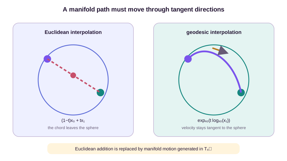
A Riemannian metric \(g_x\) supplies an inner product on each tangent space. It defines the local squared norm

\[\lVert v\rVert_{g_x}^2=g_x(v,v)\]

and therefore lengths of curves, angles, distances, and shortest paths. The metric is part of the model specification: changing it changes which paths count as straight and how errors along different directions are weighted.

Exponential and logarithmic maps replace addition and subtraction

The exponential map starts from a point and a tangent velocity:

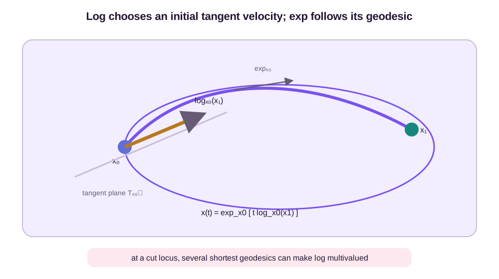
\[\operatorname{Exp}_x:T_x\mathcal{M}\to\mathcal{M}.\]

The point \(\operatorname{Exp}_x(v)\) is reached after following the geodesic that begins at \(x\) with velocity \(v\) for unit time. In Euclidean space it reduces to \(\operatorname{Exp}_x(v)=x+v\).

Locally, the logarithmic map reverses this operation:

\[\operatorname{Log}_x(y) \in T_x\mathcal{M}, \qquad \operatorname{Exp}_x(\operatorname{Log}_x(y))=y.\]

It is the geometric analogue of \(y-x\). Given endpoint pair \((x_0,x_1)\), a constant-speed geodesic conditional path is

\[x_t = \operatorname{Exp}_{x_0} \left(t\operatorname{Log}_{x_0}(x_1)\right).\]

At an intermediate point, its target velocity can be written

\[u_t(x_t\mid x_1) = \frac{1}{1-t} \operatorname{Log}_{x_t}(x_1).\]

The factor \(1/(1-t)\) does not imply that the velocity actually diverges along an exact constant-speed path: the remaining log displacement shrinks proportionally to \(1-t\). Numerically, however, evaluating this quotient very near the endpoint can be ill-conditioned, so implementations often use equivalent endpoint-pair formulas or avoid sampling \(t=1\) exactly.

The Riemannian conditional flow-matching loss is now almost forced:

\[\mathcal{L}_{\mathrm{RCFM}}(\theta) = \mathbb{E} \left[ g_{x_t}\left( v_\theta(t,x_t)-u_t(x_t\mid x_0,x_1), v_\theta(t,x_t)-u_t(x_t\mid x_0,x_1) \right) \right].\]

Both vectors are compared in the same tangent space \(T_{x_t}\mathcal{M}\). Chen and Lipman show how this construction extends flow matching to general geometries without computing density divergences during training (Chen & Lipman, 2024).

One quarter-circle through the entire interface

The unit sphere makes every replacement explicit. Take

\[x_0=(1,0,0), \qquad x_1=(0,1,0).\]

Their geodesic separation is \(\vartheta=\arccos(x_0^{\mathsf T}x_1)=\pi/2\). Away from the antipode, the sphere logarithm is

\[\operatorname{Log}_x(y) = \frac{\vartheta}{\sin\vartheta} \left(y-\cos\vartheta\,x\right), \qquad \vartheta=\arccos(x^{\mathsf T}y).\]

At \(x_0\), orthogonality makes this

\[\operatorname{Log}_{x_0}(x_1) = \frac{\pi}{2}(0,1,0).\]

The vector is attached to \(x_0\) and is tangent because its dot product with \(x_0\) vanishes. The sphere exponential for a tangent vector \(v\) is

\[\operatorname{Exp}_x(v) = \cos(\lVert v\rVert)x + \sin(\lVert v\rVert) \frac{v}{\lVert v\rVert}.\]

Substituting the logarithm yields the quarter-circle

\[x_t = \left( \cos\frac{\pi t}{2}, \sin\frac{\pi t}{2}, 0 \right).\]

Differentiation gives its constant-speed tangent target,

\[u_t = \dot x_t = \frac{\pi}{2} \left( -\sin\frac{\pi t}{2}, \cos\frac{\pi t}{2}, 0 \right), \qquad \lVert u_t\rVert=\frac{\pi}{2}.\]

At the midpoint,

\[x_{1/2} = \frac{1}{\sqrt2}(1,1,0), \qquad u_{1/2} = \frac{\pi}{2\sqrt2}(-1,1,0) \approx(-1.1107,1.1107,0).\]

The endpoint form agrees. The remaining logarithm is

\[\operatorname{Log}_{x_{1/2}}(x_1) = \frac{\pi}{4\sqrt2}(-1,1,0),\]

and division by \(1-t=1/2\) returns exactly \(u_{1/2}\). The base point changed from \(x_0\) to \(x_{1/2}\), so the two log vectors cannot be equated as ambient arrays without accounting for where they live.

Suppose an ambient network emits \(\widetilde v=(0,2,1)\) at the midpoint. The tangent projection is

\[v = (\mathbf I-x_{1/2}x_{1/2}^{\mathsf T})\widetilde v = (-1,1,1).\]

Indeed, \(x_{1/2}^{\mathsf T}v=0\). With the sphere’s induced metric, the squared regression error is the ambient squared norm of the tangent difference:

\[\lVert v-u_{1/2}\rVert_{g_{x_{1/2}}}^2 = 2\left(1-\frac{\pi}{2\sqrt2}\right)^2+1 \approx1.0245.\]

The projection makes the output legal; it does not make it accurate. The unit normal component of the original network output disappears entirely from the tangent target, while the remaining error is measured at the midpoint’s metric.

An intrinsic step and two ambient approximations

Now advance from \(t=1/2\) by \(\Delta t=1/4\) using the exact target. The intrinsic exponential step is

\[x_{3/4}^{\mathrm{Exp}} = \operatorname{Exp}_{x_{1/2}} \left(\frac14u_{1/2}\right) = \left(\cos\frac{3\pi}{8},\sin\frac{3\pi}{8},0\right) \approx(0.3827,0.9239,0).\]

Ambient Euler instead returns

\[y = x_{1/2}+\frac14u_{1/2} \approx (0.4294,0.9848,0).\]

Its norm is \(\sqrt{1+(\pi/8)^2}\approx1.0743\), so it misses the sphere by about \(0.0743\) in radial norm. Normalizing \(y\) gives a valid retraction. The retracted step rotates by \(\arctan(\pi/8)\approx0.3742\) radians rather than the intrinsic \(\pi/8\approx0.3927\). Its geodesic error is therefore about \(0.0185\) radians after one step.

Both errors vanish as \(\Delta t\to0\), but at different orders and with different constants. Projection or normalization repairs the constraint after an ambient step; it does not reproduce the exponential map exactly. Repeating the discrepancy over many learned, nonconstant steps can alter the sampled endpoint even when every intermediate point has unit norm.

Worked examples: a rotation and a periodic angle

For \(SO(3)\), tangent directions may be represented by skew-symmetric matrices. Let \(R_0=I\) and let \(R_1\) be a rotation by angle \(\omega=2\pi/3\) around the \(z\)-axis. Write

\[\Omega = \omega \begin{bmatrix} 0&-1&0\\ 1&0&0\\ 0&0&0 \end{bmatrix}.\]

Then \(R_1=\exp(\Omega)\) and the geodesic path is

\[R_t=R_0\exp(t\Omega)=\exp(t\Omega).\]

At \(t=1/2\) the orientation has rotated by \(60^\circ\), and every \(R_t\) remains orthogonal with determinant one. The failure of entrywise interpolation is numerical, not merely formal. For the \(120^\circ\) endpoint,

\[R_1 = \begin{bmatrix} -1/2&-\sqrt3/2&0\\ \sqrt3/2&-1/2&0\\ 0&0&1 \end{bmatrix}.\]

Its entrywise midpoint is

\[A = \frac{I+R_1}{2} = \begin{bmatrix} 1/4&-\sqrt3/4&0\\ \sqrt3/4&1/4&0\\ 0&0&1 \end{bmatrix}.\]

The first two columns have norm \(1/2\), so

\[A^{\mathsf T}A = \operatorname{diag}(1/4,1/4,1), \qquad \det A=1/4.\]

The matrix shrinks the \(xy\) plane; it is neither orthogonal nor a rotation. By contrast, \(\exp(\Omega/2)\) is the \(60^\circ\) rotation with \(R_{1/2}^{\mathsf T}R_{1/2}=I\) and determinant one. Projecting \(A\) back to \(SO(3)\) by a polar decomposition happens to recover the midpoint in this symmetric example, but that projection is an additional numerical operation with its own branch and differentiation behavior.

At angle \(\pi\), the axis–angle logarithm reaches a cut locus. A rotation by \(\pi\) around axis \(n\) is also represented by angle \(-\pi\) around the same axis, or by \(\pi\) around \(-n\). The endpoint is valid, but the principal logarithm cannot choose a globally continuous target across that set.

For a torsion angle \(\phi\in S^1\), the shortest signed displacement is

\[\Delta(\phi_0,\phi_1) = \operatorname{atan2} \left( \sin(\phi_1-\phi_0), \cos(\phi_1-\phi_0) \right).\]

The geodesic is

\[\phi_t = \left(\phi_0+t\Delta\right)\bmod 2\pi.\]

Take \(\phi_0=170^\circ\) and \(\phi_1=-170^\circ\). Ordinary subtraction suggests a \(-340^\circ\) journey. The circular logarithm gives \(\Delta=20^\circ\) and correctly crosses the periodic boundary.

The branch jump near the antipode is large even when the endpoints are close as points on the circle. Fix \(\phi_0=0\). Two targets at \(\phi_1^+=\pi-\epsilon\) and \(\phi_1^-=-\pi+\epsilon\) are separated on \(S^1\) by only \(2\epsilon\), but their principal logarithms are

\[\Delta^+=\pi-\epsilon, \qquad \Delta^-=-\pi+\epsilon.\]

The regression targets differ by \(2\pi-2\epsilon\). With \(\epsilon=0.01\) radians, moving the endpoint by only \(0.02\) radians across the branch changes the target by about \(6.263\) radians. At exactly \(\epsilon=0\), clockwise and counterclockwise geodesics tie. A network trained with the principal branch sees a discontinuous label even though the physical endpoint varies continuously.

One response is to change the path or representation rather than ask a smooth network to fit the jump. Wrapped conditional distributions can average branches; a sine–cosine embedding removes the coordinate discontinuity but still does not select a unique shortest tangent at the antipode. Molecular conformer models exploit the toroidal geometry of collections of torsions rather than treating each angle as an unconstrained real coordinate (Jing et al., 2022).

Probability still obeys a continuity equation

Let \(d\mathrm{vol}_g\) be the Riemannian volume measure and let \(p_t\) denote density with respect to that measure. Probability conservation becomes

\[\partial_t p_t + \operatorname{div}_{\mathcal{M}}(p_tu_t) =0.\]

In local coordinates with metric matrix \(G(x)=[g_{ij}(x)]\),

\[\operatorname{div}_{\mathcal{M}} u = \frac{1}{\sqrt{\lvert G\rvert}} \sum_i \partial_{x^i} \left( \sqrt{\lvert G\rvert} u^i \right).\]

The factor \(\sqrt{\lvert G\rvert}\) corrects for how coordinate volume changes across the manifold. Omitting it treats chart coordinates as though they had uniform Euclidean volume, which generally gives the wrong density dynamics. Riemannian continuous normalizing flows use precisely this geometric change-of-variables structure (Mathieu & Nickel, 2020).

Constant coordinate speed can still expand volume

Spherical coordinates expose the missing factor. On the unit sphere, away from the poles,

\[ds^2=d\vartheta^2+\sin^2\vartheta\,d\varphi^2, \qquad G = \begin{bmatrix} 1&0\\0&\sin^2\vartheta \end{bmatrix}, \qquad \sqrt{\lvert G\rvert}=\sin\vartheta.\]

Consider the local vector field with constant polar coordinate speed \(u^\vartheta=a\) and \(u^\varphi=0\). A flat-coordinate calculation would report \(\partial_\vartheta a+\partial_\varphi0=0\). Riemannian divergence gives

\[\operatorname{div}_{S^2}u = \frac{1}{\sin\vartheta} \partial_\vartheta(\sin\vartheta\,a) = a\cot\vartheta.\]

The field has positive divergence in the northern hemisphere because equal increments in \(\vartheta\) sweep through latitude bands with changing circumference. It has negative divergence in the southern hemisphere and zero divergence at the equator. The coordinate components are constant; the physical cross-sectional area is not.

Take \(a=0.2\) radians per unit time at \(\vartheta=\pi/3\). Then

\[\operatorname{div}_{S^2}u = 0.2\cot\frac{\pi}{3} = \frac{0.2}{\sqrt3} \approx0.1155.\]

Along a deterministic flow, density relative to Riemannian volume obeys the instantaneous change-of-variables identity

\[\frac{d}{dt}\log p_t(x_t) = -\operatorname{div}_{S^2}u_t(x_t).\]

Over a short interval \(\Delta t=0.1\) in which the divergence is approximately constant, the log density changes by about \(-0.01155\), a density factor \(e^{-0.01155}\approx0.9885\). The flat-coordinate divergence would predict no change. Exact integration would evaluate \(a\cot\vartheta_t\) along the moving trajectory rather than freeze it; the short-step calculation isolates the volume-form correction.

The choice of reference measure is therefore observable in likelihoods. If a chart density \(q(\vartheta,\varphi)\) is defined relative to \(d\vartheta\,d\varphi\) while \(p\) is defined relative to surface area, then

\[q(\vartheta,\varphi) = p(\vartheta,\varphi)\sin\vartheta.\]

Confusing \(p\) and \(q\) introduces the missing \(\log\sin\vartheta\) term and makes a uniform sphere look nonuniform in coordinates.

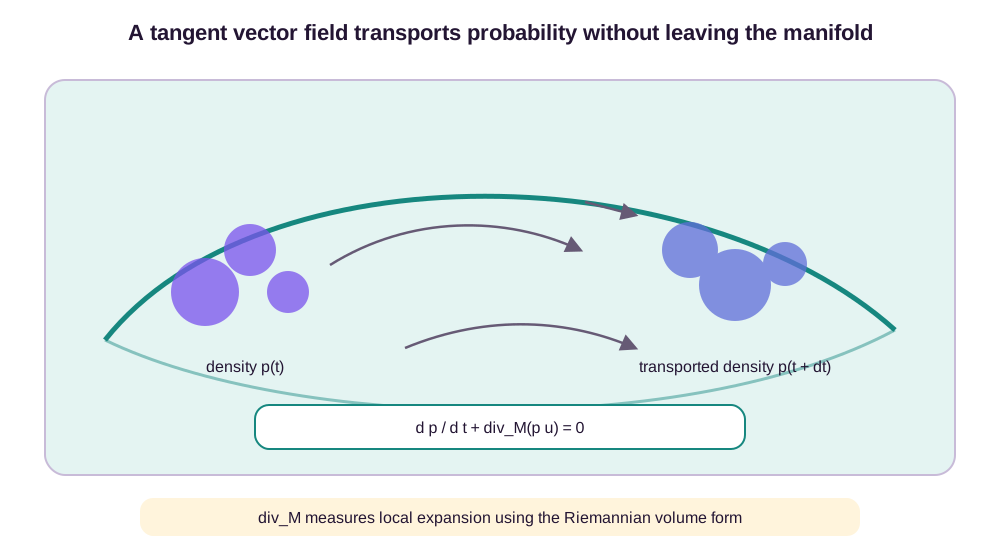
This separates two tasks that are often conflated. Sampling only requires solving the manifold ODE. Exact likelihood evaluation requires integrating the Riemannian divergence along trajectories and using densities relative to the same declared base volume. Flow matching avoids divergence during training, not necessarily during density evaluation.

Equivariance constrains the vector field

Manifold geometry and data symmetry are related but distinct. The fact that rotations live on \(SO(3)\) describes the state space. The claim that rotating an entire molecule should rotate a generated structure describes an external group action.

Let a group element \(h\) act on \(\mathcal{M}\) by an isometry \(\rho_h\). Its differential

\[d\rho_h\big\rvert_x: T_x\mathcal{M} \to T_{\rho_h(x)}\mathcal{M}\]

maps tangent velocities between the appropriate tangent spaces. A vector field is equivariant when

\[v_\theta(t,\rho_h(x)) = d\rho_h\big\rvert_x v_\theta(t,x).\]

If the base distribution and conditional-path construction respect the same action, integrating this field commutes with the action. This is the continuous-time analogue of equivariant message passing. In protein generation, FoldFlow combines flow matching with the geometry and symmetry of residue frames in \(SE(3)\) (Bose et al., 2024).

The commutation claim follows from ODE uniqueness. Let \(\Psi_{t,0}(x)\) denote the flow beginning at \(x\) at time zero, and assume the vector field is regular enough that the initial-value problem has a unique solution. Define

\[y_t = \rho_h\!\left(\Psi_{t,0}(x)\right).\]

The curve \(\Psi_{t,0}(x)\) has velocity in \(T_{\Psi_{t,0}(x)}\mathcal M\). Differentiating through the action maps that velocity to the correct new base point:

\[\begin{aligned} \dot y_t &= d\rho_h\big\rvert_{\Psi_{t,0}(x)} v_t\!\left(\Psi_{t,0}(x)\right)\\ &= v_t\!\left( \rho_h(\Psi_{t,0}(x)) \right) =v_t(y_t). \end{aligned}\]

The second equality is vector-field equivariance. The initial condition is \(y_0=\rho_h(x)\). Therefore \(y_t\) and \(\Psi_{t,0}(\rho_h(x))\) solve the same ODE with the same initial condition. Uniqueness gives

\[\rho_h\circ\Psi_{t,0} = \Psi_{t,0}\circ\rho_h.\]

Equivariance of the instantaneous field has become equivariance of the finite-time flow map. If solutions are nonunique, the last step fails: field equivariance only maps a solution to another valid solution, not necessarily to the solver-selected one. A numerical method can also break exact commutation unless its update respects the group action. For example, a Lie-group exponential update inherits left-action equivariance under standard conditions, whereas chart clipping may depend on the chosen coordinates.

The base distribution determines whether this equivariant map produces an invariant or equivariant distribution. If \(p_0\) is invariant under \(\rho_h\), then pushing it through the commuting flow yields invariant marginals. If the base is conditioned on an external frame, the map can commute perfectly while the distribution retains that frame bias. Architecture, base, conditional paths, and solver each occupy a separate line of the symmetry contract.

Molecular state spaces are product manifolds

A molecule rarely lives on one homogeneous manifold. A residue frame contains a translation in \(\mathbb{R}^3\) and an orientation in \(SO(3)\). Side-chain torsions live on copies of \(S^1\). A schematic protein state space is therefore

\[\mathcal{M} = \left(\mathbb{R}^3\times SO(3)\right)^N \times \left(S^1\right)^K.\]

Its tangent space factors componentwise:

\[T_x\mathcal{M} \cong \prod_{i=1}^{N} \left(\mathbb{R}^3\times\mathfrak{so}(3)\right) \times\mathbb{R}^K.\]

A product metric can weight these parts:

\[\lVert u\rVert_g^2 = w_x\lVert u_x\rVert^2 +w_R\lVert u_R\rVert^2 +w_\phi\lVert u_\phi\rVert^2.\]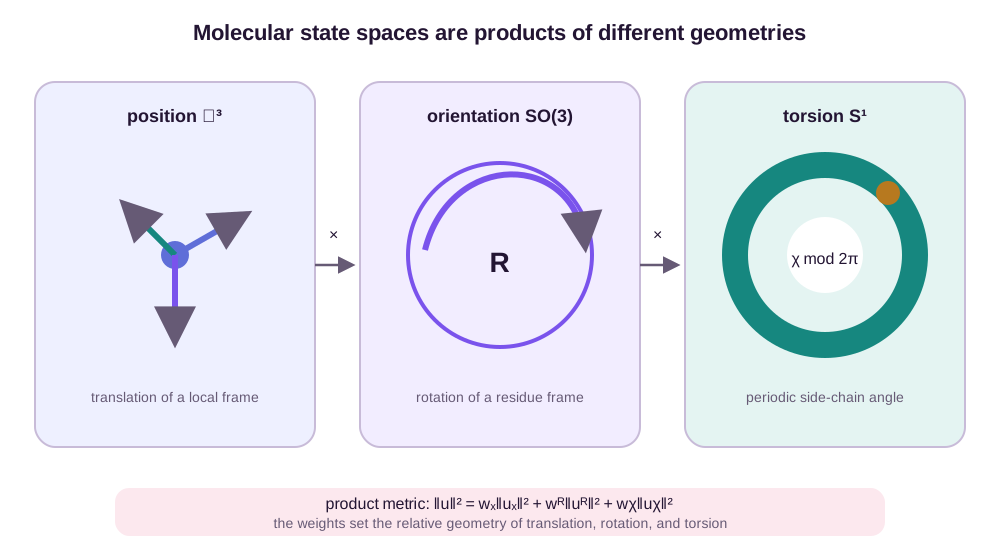

Those weights carry units. If translations are measured in angstroms and angles in radians, a dimensionless squared norm can use

\[w_x=\frac{1}{\sigma_x^2}, \qquad w_R=\frac{1}{\sigma_R^2}, \qquad w_\phi=\frac{1}{\sigma_\phi^2},\]

where the three \(\sigma\) values are declared physical scales. For \(\sigma_x=0.5\ \text{\AA}\), \(\sigma_R=0.25\) radians, and \(\sigma_\phi=0.5\) radians, a velocity error of \(1\ \text{\AA}\), \(0.2\) radians, and \(0.5\) radians contributes

\[4(1)^2+16(0.2)^2+4(0.5)^2 = 4+0.64+1 =5.64.\]

Without declared scales, adding squared lengths and squared angles has no physical exchange rate. The weights decide which component errors dominate regression and adaptive-solver tolerances.

Constant factor weights have a narrower geometric effect than is sometimes claimed. On a direct product with no cross terms, multiplying each factor metric by a positive constant leaves that factor’s Levi–Civita connection unchanged. For fixed paired endpoints, the component geodesic curves and their affine-time parameterizations therefore remain the same; the total product distance and loss change. State-dependent weights or cross-component metric terms would change the geodesic equations themselves.

The endpoint coupling matters too. Independent pairs yield simple training, but their geodesics may cross low-density regions or take unnecessarily long paths. Approximate optimal-transport couplings can shorten conditional paths and reduce target variance, at the cost of solving a batch-level matching problem. On products, the metric weights directly affect which endpoints are paired.

Consider one base state and two candidate data endpoints. Candidate A differs by \(0.2\ \text{\AA}\) in translation and \(0.8\) radians in rotation. Candidate B differs by \(1.0\ \text{\AA}\) and \(0.1\) radians. Ignore torsions for this comparison. With \(w_x=1\) and \(w_R=0.5\), their squared costs are

\[c_A=0.2^2+0.5(0.8)^2=0.36, \qquad c_B=1^2+0.5(0.1)^2=1.005,\]

so an optimal coupling prefers A. Raising the rotation weight to \(w_R=4\) gives

\[c_A=0.04+4(0.64)=2.60, \qquad c_B=1+4(0.01)=1.04,\]

and the coupling switches to B. The component geodesic from the base to A did not change; the selected endpoint did. This separates three effects that are easy to conflate: constant product weights rescale loss and distance, those rescaled distances can alter endpoint coupling, and only more general metric changes alter each fixed-endpoint component geodesic.

Topology and numerics are part of the model

The geodesic formula is elegant, but several complications determine whether it works in practice.

There may be no global logarithm. On a sphere, the antipode of \(x\) has infinitely many shortest geodesics from \(x\). On \(SO(3)\), rotations by angle \(\pi\) sit at the analogous ambiguity. A chosen principal logarithm is discontinuous across the cut locus. These sets may have zero volume, yet samples near them can still produce large target variation.

The base distribution is geometry-dependent. There is no universal manifold Gaussian. Compact homogeneous spaces admit a uniform base; other settings use wrapped distributions, heat kernels, or a distribution defined through charts or an embedding. The base affects both coverage and how difficult the learned transport must be.

A generic ODE step can leave the manifold. The geometric Euler update

\[x_{t+\Delta t} \approx \operatorname{Exp}_{x_t} \left(\Delta t\,v_\theta(t,x_t)\right)\]

respects the manifold by construction. Exact exponential maps can be expensive, so implementations use retractions, projection, Lie-group integrators, or chart-based solvers. Projection is simple but can distort the intended vector field; charts can introduce singularities; repeated matrix exponentials can dominate runtime.

Curvature limits comfortable step sizes. A tangent-space linearization is only local. Large solver steps are less reliable where curvature is high or the vector field changes rapidly. Adaptive solvers reduce error but make the number of neural evaluations unpredictable.

Topology cannot be wished away by coordinates. Unwrapping an angle to the real line introduces an artificial boundary. Representing a rotation by a quaternion introduces a double cover, because \(q\) and \(-q\) describe the same rotation. Every parameterization trades one difficulty for another; the model, loss, and solver must agree on that choice.

The representation and solver must share a state space

Quaternions make the contract concrete. Unit quaternions live on \(S^3\), and the map to \(SO(3)\) identifies \(q\) with \(-q\). A Euclidean loss \(\lVert q_1-q_0\rVert^2\) is therefore representation-dependent: two arrays can be antipodes in \(\mathbb R^4\) and still describe the same physical rotation. A sign-invariant endpoint comparison uses

\[d_{\mathrm{quat}}(q_0,q_1) = 2\arccos\left(\lvert q_0^{\mathsf T}q_1\rvert\right),\]

which returns the physical rotation angle in \([0,\pi]\). The absolute value chooses the nearer lift. That choice is itself nondifferentiable when the inner product is zero, corresponding to the \(\pi\) cut locus in \(SO(3)\).

One common implementation flips the endpoint sign so that \(q_0^{\mathsf T}q_1\geq0\) before spherical interpolation. This shortens each paired path on \(S^3\), but independent sign decisions across nearby training pairs can create label switches near orthogonality. Enforcing a continuous quaternion sign over an entire dataset is impossible around every nontrivial loop because the double cover has no global continuous section. The discontinuity was moved from matrices or axis–angle coordinates into lift selection; it was not removed.

Charts trade the same global issue for local coordinates. A chart-based network may output an ordinary vector and use a standard ODE solver until the trajectory approaches the chart boundary. Switching charts then requires transforming both the state and velocity with the chart-transition Jacobian. Clipping the coordinate without transforming the vector field changes the ODE. An atlas can cover the manifold, but the numerical method must decide when and how to switch.

Retractions offer a controlled local approximation. A map \(R_x:T_x\mathcal M\to\mathcal M\) is a first-order retraction when \(R_x(0)=x\) and its derivative at zero is the identity on \(T_x\mathcal M\). This guarantees agreement with the exponential map to first order, not at finite step size. The sphere normalization used above is a retraction: \(R_x(v)=(x+v)/\lVert x+v\rVert\) for \(x^{\mathsf T}v=0\). Its one-step angular error \(\pi/8-\arctan(\pi/8)\approx0.0184\) showed the missing higher-order geometry explicitly.

Adaptive error control also needs a geometric norm. Subtracting two candidate rotation matrices entrywise measures embedding error, while a logarithm such as \(\lVert\operatorname{Log}_{R_a}(R_b)\rVert\) measures intrinsic rotation error. Either can define a practical tolerance locally, but the reported tolerance must match the chosen measure. A solver that controls ambient quaternion error without identifying \(q\sim-q\) can reject a physically exact step merely because two equivalent lifts have opposite signs.

Base distributions inherit the topology

The base distribution cannot be selected independently of these choices. Uniform measure is natural on compact homogeneous factors such as \(S^1\) and \(SO(3)\), but it may be too far from structured molecular data for an easy transport. A concentrated wrapped or heat-kernel base shortens typical paths but can under-cover distant modes. On a noncompact translation factor, a Gaussian needs a scale and a choice of frame; removing center of mass changes the dimension and introduces a constraint subspace.

Product bases introduce correlations as well. Sampling residue orientations uniformly and translations independently may be tractable, but it does not encode steric feasibility or chain connectivity. The learned field must repair those mismatches along its path. A more structured base can reduce transport difficulty while making exact sampling or likelihood evaluation harder. “Simple base” means simple with respect to the declared manifold and measure, not simply a standard normal array in an embedding space.

The point of the geometry

Geometric flow matching is not ordinary flow matching followed by a projection at the end. The geometry determines the valid velocity at every time, the conditional path used as supervision, the norm in the loss, the volume form in the continuity equation, and the numerical update used for sampling.

The implementation can be audited as one contract:

Decision	Mathematical object supplied	Failure if left implicit
State and representation	Manifold, quotient, embedding, or atlas	Equivalent physical states receive different losses or invalid updates
Base distribution	Density relative to a declared volume measure	Sampling and likelihood use incompatible normalizations
Conditional coupling and path	Endpoint law plus tangent velocity at every base point	Paths cross cut loci, labels jump, or the marginal path is not the intended one
Metric	Tangent inner product with physical scales	Translation, rotation, and torsion errors are combined without units
Symmetry	External action and its tangent differential	The field or numerical flow depends on an arbitrary frame
Cut-locus policy	Branch, mixture, alternate path, or excluded region	Principal-log targets become discontinuous near ambiguous endpoints
Rotation coordinates	Matrix, quaternion lift, or local chart	Orthogonality, double-cover, or chart-boundary errors enter unnoticed
Solver	Exponential, retraction, Lie-group, or chart update with a geometric tolerance	States leave the manifold or follow a systematically altered path

The quarter-circle shows how these lines interact. Its logarithm selected a unique tangent because the endpoints were not antipodal. The induced sphere metric measured the midpoint error. The exponential update landed at the exact three-quarter point, while normalized Euler incurred a quantified angular bias. The sphere volume factor then changed likelihood even for a constant coordinate-speed field. Rotating the initial state commuted with the exact flow only because the vector field transformed between the correct tangent base points and the ODE solution was unique.

None of those conclusions follows from replacing \(x_1-x_0\) by a logarithm in one equation. The base measure, loss, symmetry action, endpoint coupling, and solver are part of the generative model. Flow matching removes trajectory simulation from training target construction. It does not remove the topology of the generated space, nor the numerical approximation used to traverse it.

References

1. Lipman, Y., Chen, R. T. Q., Ben-Hamu, H., Nickel, M., & Le, M. (2023). Flow Matching for Generative Modeling. ICLR. ↩
2. Chen, R. T. Q., & Lipman, Y. (2024). Flow Matching on General Geometries. ICLR. ↩
3. Mathieu, E., & Nickel, M. (2020). Riemannian Continuous Normalizing Flows. NeurIPS. ↩
4. Bose, A. J. et al. (2024). SE(3)-Stochastic Flow Matching for Protein Backbone Generation. ICLR. ↩
5. Jing, B., Corso, G., Chang, J., Barzilay, R., & Jaakkola, T. (2022). Torsional Diffusion for Molecular Conformer Generation. NeurIPS. ↩

---

Figure provenance. All four geofm_ diagrams are original SVG illustrations generated by scripts/generate_geofm_figures.py. They synthesize standard Riemannian geometry and flow-matching constructions described in the cited primary literature; no third-party artwork is reproduced.