Note: This post introduces Generative Flow Networks (GFlowNets) for ML researchers who already think in terms of probability distributions and sampling. It follows the probabilistic view from a KAIST talk in June 2024 and uses RL mainly as notation for sequential construction. For the original framing, see Emmanuel Bengio's Introduction to GFlowNets and Yoshua Bengio's GFlowNet Tutorial.
Introduction
Suppose you want to generate a molecule that binds to a target protein. You have a reward function \(R(x)\) that scores how well molecule \(x\) binds. The standard RL approach maximizes expected reward, but that tends to converge to one high-reward molecule and ignore other good candidates.
In scientific discovery, diversity is essential. Proxy reward functions are imprecise; the top-scoring molecule under the proxy may fail experimentally. The safer strategy is to cast a wide net: generate many diverse candidates that score well, then filter them in the lab.
GFlowNets address this by sampling objects proportionally to their reward (Bengio et al., 2021). Instead of finding \(x^* = \arg\max_x R(x)\), a GFlowNet learns a policy that generates \(x\) with probability proportional to \(\exp R(x)\). If molecule A has reward 4 and molecule B has reward 2, A is sampled \(e^4 / e^2 \approx 7.4\) times more often than B, but B is still generated regularly. This is an energy-based (Boltzmann) distribution, the same type that appears in statistical mechanics and Bayesian inference.
Part I: The Goal
Sampling from Energy-Based Distributions
GFlowNet is a generative framework for sampling combinatorial objects from an energy-based (Boltzmann) distribution:
Target distribution. The goal is to learn a policy \(p_\theta(x)\) that approximates
\[p^*(x) = \frac{\exp R(x)}{Z}, \qquad Z = \sum_{x \in \mathcal{X}} \exp R(x)\]where \(R(x)\) is a reward function (or negative energy), \(\mathcal{X}\) is a finite set of objects, and \(Z\) is the partition function — a normalizing constant that ensures the probabilities sum to one.
We can evaluate \(R(x)\) for any given object \(x\), for example by running a docking simulation, but we cannot enumerate all objects to compute \(Z\). Unlike VAEs or diffusion models, the model learns directly from the reward function, not from a dataset of samples from \(p^*(x)\).
Amortized Sampling
MCMC methods such as Metropolis-Hastings, Langevin dynamics, and HMC can sample from \(p^*(x)\) without knowing \(Z\), but each run produces a single correlated chain of samples. When we need repeated samples from the same distribution, or from many related distributions, rerunning MCMC from scratch is wasteful.
GFlowNets perform amortized sampling: they invest upfront computation to train a neural network (the forward policy), and then sampling is a single forward pass through the network — fast and parallelizable. This is the same idea behind amortized variational inference, where an encoder network replaces per-datapoint optimization. The upfront training cost is large, but inference at deployment time is cheap.
In probabilistic-ML terms, GFlowNets are amortized MCMC for combinatorial spaces: train once, sample forever, with the learned policy replacing the Markov chain.
Why Not RL?
RL maximizes expected cumulative reward. It finds the single best action sequence, or a narrow set of near-optimal ones. GFlowNets solve a different problem: sampling proportionally to reward. The two are related but distinct:
- Similar: Both use interactive training with a reward function and learn a policy through trial and error.
- Different: RL converges to the mode; GFlowNets converge to the full distribution.
For scientific discovery, mode-seeking is dangerous. If the reward function is a learned proxy for binding affinity, its top-scoring molecule may not bind well in the lab. We want many diverse candidates so that some can succeed even when others fail experimentally.
Maximum entropy RL comes closer — it augments the reward with an entropy bonus that encourages the policy to spread probability mass across trajectories. GFlowNets turn out to be equivalent to MaxEnt RL with a specific reward shaping, but they target a distribution over terminal objects rather than trajectories. Part V returns to this connection.
Part II: GFlowNet Basics
DAG of States
GFlowNets construct objects step by step, like assembling a molecule atom by atom. The construction process is represented as a directed acyclic graph (DAG): a graph with directed edges and no cycles, so every path eventually terminates. The DAG has three types of nodes:
- A single initial state \(s_0\), such as an empty molecule.
- Intermediate states represent partially constructed objects (e.g., a molecule with some atoms added).
- Terminal states \(x \in \mathcal{X}\) are the completed objects.
Each edge \((s_{t-1}, s_t)\) in the DAG represents an action, such as adding an atom, appending an amino acid, or placing a node. Multiple trajectories can lead to the same terminal object \(x\), because different construction orders can produce the same result.


Forward Policy
The forward policy \(p_\mathrm{F}(s_t \mid s_{t-1})\) is a learned distribution over next states given the current state — a neural network that looks at the current partial object and decides what to add next. A trajectory \(\tau = (s_0, s_1, \ldots, s_T = x)\) is a complete path from the initial state to a terminal state. Its probability is the product of all transition probabilities along the path:
\[p_\mathrm{F}(\tau) = \prod_{t=1}^{T} p_\mathrm{F}(s_t \mid s_{t-1})\]The probability of generating a specific object \(x\) is the sum over all trajectories that end at \(x\):
\[p_\mathrm{F}(x) = \sum_{\tau \in \mathcal{T}(x)} p_\mathrm{F}(\tau)\]where \(\mathcal{T}(x)\) is the set of all trajectories that terminate at \(x\). For example, a molecule with three atoms A, B, C can be built as A→B→C or A→C→B or B→A→C, and so on — all producing the same molecule \(x\). The total probability of generating \(x\) is the sum over all these construction orders.

The Key Difficulty
We want \(p_\mathrm{F}(x) \approx p^*(x)\) for every object \(x\), but computing \(p_\mathrm{F}(x)\) requires summing over all trajectories \(\mathcal{T}(x)\). For a molecule with 20 atoms, the number of construction orders can be astronomically large, making this sum intractable.
GFlowNets sidestep this by replacing object-level matching with trajectory-level matching. Instead of asking whether the probability of each object \(x\) matches \(p^*(x)\), we ask whether each trajectory under the forward policy matches a target trajectory distribution. If trajectory probabilities match, object probabilities match automatically: \(p_\mathrm{F}(x) = \sum_\tau p_\mathrm{F}(\tau)\), so matching each trajectory also matches the sum.
Backward Policy
To define a target distribution over trajectories, we need a way to decompose each terminal object \(x\) into a trajectory. The backward policy \(p_\mathrm{B}(s_{t-1} \mid s_t)\) does this: given a state, it assigns probabilities to its parent states in the DAG. Starting from a terminal state \(x\) and repeatedly sampling parents, we trace a path back to the initial state \(s_0\) — a trajectory in reverse.
The backward policy, combined with the reward, defines the target distribution over trajectories:
\[p_\mathrm{B}(\tau) \propto \exp R(x) \prod_{t=1}^{T} p_\mathrm{B}(s_{t-1} \mid s_t)\]A trajectory leading to a high-reward terminal state gets high probability; the backward policy determines how that probability is split among the different construction orders for \(x\). The backward policy can be fixed (e.g., uniform over parents) or learned jointly with the forward policy.

A Worked Example: Uniform Backward Policy
Consider a simple DAG with three terminal states \(x_1, x_2, x_3\) and unnormalized target weights \(\exp R(x_1) = 4\), \(\exp R(x_2) = 2\), \(\exp R(x_3) = 1\). With a uniform backward policy, and assuming each state has exactly one parent so \(p_\mathrm{B} = 1\) on every edge, each terminal state has exactly one backward trajectory. Each trajectory’s target probability is proportional to \(\exp R(x)\): \(p_\mathrm{B}(\tau_1) \propto 4\), \(p_\mathrm{B}(\tau_2) \propto 2\), \(p_\mathrm{B}(\tau_3) \propto 1\). The total is \(4 + 2 + 1 = 7\), so the forward policy must route 4/7 of its probability toward \(x_1\), 2/7 toward \(x_2\), and 1/7 toward \(x_3\).

A Worked Example: Non-Uniform Backward Policy
What if the backward policy is non-uniform? Suppose \(x_2\) has two parents \(s_1\) and \(s_2\), and we set \(p_\mathrm{B}(s_1 \mid x_2) = p_\mathrm{B}(s_2 \mid x_2) = 0.5\). Now there are four trajectories instead of three, because \(x_2\) can be reached through either \(s_1\) or \(s_2\). The backward policy splits \(x_2\)’s weight of \(\exp R(x_2) = 2\) across the two paths: each trajectory through \(x_2\) gets target probability proportional to \(2 \times 0.5 = 1\). The forward policy adjusts by routing more probability through \(s_2\), because \(s_2\) serves as a waypoint to both \(x_2\) and \(x_3\).

Flows
We want \(p_\mathrm{F}(\tau) \approx p_\mathrm{B}(\tau)\), but \(p_\mathrm{B}(\tau)\) is defined only up to a normalizing constant, the \(\propto\) in the equation above. We do not know the partition function \(Z\), so we cannot compute the actual probability \(p_\mathrm{B}(\tau)\).
The solution is to work with unnormalized densities instead of probabilities. We multiply both sides by their respective normalizing constants and match the unnormalized quantities directly:
\[f_\mathrm{F}(\tau) = Z_\theta \prod_{t=1}^{T} p_\mathrm{F}(s_t \mid s_{t-1}) \approx \exp R(x) \prod_{t=1}^{T} p_\mathrm{B}(s_{t-1} \mid s_t) = f_\mathrm{B}(\tau)\]Here \(Z_\theta\) is a trainable scalar, the model’s estimate of the partition function. The left side \(f_\mathrm{F}(\tau)\) is the forward flow (unnormalized forward probability), and the right side \(f_\mathrm{B}(\tau)\) is the backward flow (unnormalized backward probability). These trajectory-wise unnormalized densities are called flows, hence the name Generative Flow Network.
Part III: Training Objectives
Trajectory Balance (TB)
The trajectory balance objective (Malkin et al., 2022) directly enforces the flow-matching condition for complete trajectories. If \(f_\mathrm{F}(\tau) = f_\mathrm{B}(\tau)\), then \(\log(f_\mathrm{F} / f_\mathrm{B}) = 0\). Squaring this log-ratio gives a loss that is zero when the flows match and positive otherwise:
Trajectory Balance. For a trajectory \(\tau = (s_0, \ldots, s_T = x)\):
\[\mathcal{L}_\mathrm{TB}(\tau) = \left(\log \frac{Z_\theta \prod_{t=1}^{T} p_\mathrm{F}(s_t \mid s_{t-1})}{\exp R(x) \prod_{t=1}^{T} p_\mathrm{B}(s_{t-1} \mid s_t)}\right)^2\]The loss is zero when the forward flow \(Z_\theta \prod p_\mathrm{F}\) equals the backward flow \(\exp R(x) \prod p_\mathrm{B}\) for every trajectory.
TB is the simplest objective. It trains a single scalar \(Z_\theta\) plus the forward and backward policies. The downside is credit assignment: a single reward signal at the terminal state must propagate back through the entire construction sequence. For long trajectories, this makes learning slow — the gradient carries information about the full trajectory, and early transitions receive weak signal.

Detailed Balance (DB)
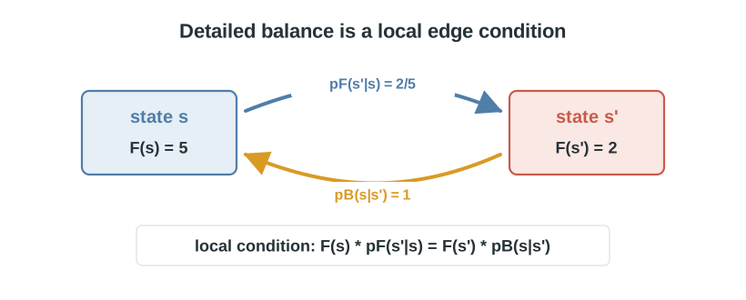
TB applies to entire trajectories, which can be long. The detailed balance objective (Bengio et al., 2023; Deleu et al., 2022) breaks this into individual transitions, one edge at a time. The idea comes from detailed balance in Markov chain theory: at equilibrium, probability flux along each edge must be equal in both directions.
Detailed Balance. For each edge \((s_{t-1}, s_t)\):
\[\mathcal{L}_\mathrm{DB}(s_{t-1}, s_t) = \left(\log \frac{f_\theta(s_{t-1}) \, p_\mathrm{F}(s_t \mid s_{t-1})}{f_\theta(s_t) \, p_\mathrm{B}(s_{t-1} \mid s_t)}\right)^2\]where \(f_\theta(s)\) is a learned state flow — the total flow through state \(s\). Boundary conditions: \(f_\theta(s_0) = Z_\theta\) and \(f_\theta(x) = \exp R(x)\) for terminal states.
DB provides local credit assignment: each transition gets its own loss signal, so early transitions receive direct feedback rather than waiting for the terminal reward. The trade-off is that the model must learn the state flow function \(f_\theta(s)\), an additional neural network that estimates how much total flow passes through each intermediate state.
Sub-Trajectory Balance (SubTB)
TB enforces balance over the full trajectory (global but weak signal); DB enforces balance over single edges (local but requires learning state flows). Sub-trajectory balance (Madan et al., 2023) interpolates between the two by enforcing balance on sub-trajectories of arbitrary length \(\ell\). For a sub-trajectory \((s_i, s_{i+1}, \ldots, s_{i+\ell})\):
Sub-Trajectory Balance. For states \(s_i, \ldots, s_{i+\ell}\) along a trajectory:
\[\mathcal{L}_\mathrm{SubTB}(s_i, \ldots, s_{i+\ell}) = \left(\log \frac{f_\theta(s_i) \prod_{t=i+1}^{i+\ell} p_\mathrm{F}(s_t \mid s_{t-1})}{f_\theta(s_{i+\ell}) \prod_{t=i+1}^{i+\ell} p_\mathrm{B}(s_{t-1} \mid s_t)}\right)^2\]where \(f_\theta(s)\) is the learned state flow. Setting \(\ell = 1\) recovers DB; setting \(i = 0\), \(\ell = T\), and using the boundary conditions \(f_\theta(s_0) = Z_\theta\), \(f_\theta(x) = \exp R(x)\) recovers TB.
In practice, SubTB sums losses over all sub-trajectories of all lengths within a sampled trajectory, optionally weighting shorter sub-trajectories more heavily. This interpolates between local credit assignment (DB) and global credit assignment (TB), and often trains more stably than either alone.
Flow Matching
An alternative to the balance conditions is flow matching (not to be confused with the flow matching used in continuous normalizing flows). This is the original training objective from the first GFlowNet paper (Bengio et al., 2021). It enforces flow conservation at each intermediate state: the total incoming flow must equal the total outgoing flow, like water in a pipe network. This is conceptually clean but requires summing over all parents and children of each state, which can be expensive for states with many neighbors.
Why These Objectives Are Easy to Optimize
GFlowNet training is simpler than the problem statement suggests. The TB loss is a squared log-ratio between two quantities we can compute for any given trajectory. This is a regression problem: fit the forward flow to the backward flow, using MSE in log-space.
Compare this with on-policy RL, where you must collect fresh trajectories with the current policy, estimate advantages with high-variance baselines, and tune clipping ratios or entropy bonuses to keep training stable. GFlowNet training looks more like offline RL or behavioral cloning: given a dataset of trajectories from a replay buffer, minimize a well-defined regression loss. There is no policy gradient, no REINFORCE estimator, and no reward-to-go. The gradient of \(\mathcal{L}_\mathrm{TB}\) with respect to policy parameters is straightforward backpropagation through log-probabilities, the same kind of computation used in a supervised sequence model.
GFlowNet training moves the difficulty from optimization to exploration. Sampling from an energy-based distribution over combinatorial objects sounds hard, but training reduces to something closer to supervised learning than to RL. The loss is easy to minimize on any given trajectory, but the model needs useful trajectories to train on.
Part IV: The Training Loop
Off-Policy Training with Replay
GFlowNet training follows an RL-style loop:
- Collect trajectories \(\{\tau^{(b)}\}_{b=1}^{B_1}\) using the current forward policy \(p_\mathrm{F}\).
- Store these trajectories in a replay buffer \(\mathcal{B}\).
- Train the forward policy on a batch \(\{\tau^{(b)}\}_{b=1}^{B_2}\) sampled from the replay buffer, minimizing \(\mathcal{L}_\mathrm{TB}\), \(\mathcal{L}_\mathrm{DB}\), or \(\mathcal{L}_\mathrm{SubTB}\).
This is an off-policy algorithm: training uses replayed trajectories, not only fresh ones. “Off-policy” means the trajectories used for training were not necessarily generated by the current policy; they may come from an earlier version stored in the replay buffer. Replay matters because reward evaluation is often expensive, such as docking simulations that take seconds per molecule. Replaying past trajectories extracts more learning signal per reward evaluation.
In practice, most implementations mix on-policy samples (fresh trajectories from the current \(p_\mathrm{F}\)) with replayed trajectories. The on-policy samples ensure the model keeps exploring new regions of the DAG, while the replay buffer provides a stable training distribution and prevents the model from forgetting high-reward regions it discovered earlier.
Exploration
A pure on-policy GFlowNet only visits states reachable under its current forward policy. If the policy has not yet discovered a high-reward region, it never trains on trajectories leading there. This is the same exploration challenge that plagues RL.
Common strategies include \(\epsilon\)-greedy exploration, tempering the forward policy, and prioritized replay buffers. In \(\epsilon\)-greedy exploration, the sampler takes a uniformly random action with probability \(\epsilon\) instead of sampling from \(p_\mathrm{F}\). Tempering raises the policy temperature to flatten the distribution and encourage more random choices. Prioritized replay oversamples high-reward trajectories so the model gets more training signal from the best discoveries.
Some recent work combines GFlowNets with local search (Kim et al., 2024): generate a candidate with the forward policy, improve it with local perturbations such as swapping one atom for another, and add the improved candidate to the replay buffer.
Backward Policy Design
The backward policy \(p_\mathrm{B}\) is a design choice with real consequences. It determines how the target distribution over trajectories decomposes reward across construction paths.
Uniform backward policy assigns equal probability to all parent states. This is the simplest option and works well when the DAG has uniform branching. But in DAGs where some states have many parents, the uniform backward policy spreads reward thinly across many trajectories, making each one a weak training signal.
Learned backward policies are trained jointly with the forward policy. The backward policy can concentrate reward on fewer trajectories, giving the forward policy a stronger signal. The downside is more parameters and potential instability from co-adaptation.
Pessimistic backward policy (PBP) biases the backward policy toward trajectories that are hard for the current forward policy — trajectories where \(p_\mathrm{F}(\tau) / p_\mathrm{B}(\tau)\) is small. This focuses training on the forward policy’s weakest regions, similar to hard example mining in supervised learning.
Evaluation
GFlowNet performance is measured along two axes:
- Reward quality: average reward of the top-\(k\) generated samples, or the fraction of samples exceeding a reward threshold.
- Diversity: number of distinct modes discovered. This is domain-specific — for molecules, it might be the number of structurally distinct scaffolds; for sequences, the number of distinct high-affinity families.
A good GFlowNet achieves high reward and high diversity. A model that finds one excellent molecule and generates it repeatedly has failed; downstream experimental validation needs many distinct candidates.
Part V: Connections to Existing Frameworks
GFlowNets sit at the intersection of maximum-entropy RL, variational inference, and path-space generative modeling. Their target differs from standard RL: standard RL usually wants a high-reward action sequence, while GFlowNets want a distribution over terminal objects, with probability proportional to \(\exp R(x)\).
Maximum-Entropy RL
The RL connection becomes precise once the backward policy is fixed. The backward policy lifts the terminal target over objects into a target over complete trajectories:
\[q_\mathrm{B}(\tau) = \frac{\exp R(x)}{Z} \prod_{t=1}^{T} p_\mathrm{B}(s_{t-1} \mid s_t)\]where \(\tau = (s_0, \ldots, s_T = x)\). The forward policy should match this path distribution. Equivalently, the forward policy solves a maximum-entropy RL problem whose terminal reward is \(R(x)\) and whose intermediate shaped reward is
\[r(s_{t-1}, s_t) = \log p_\mathrm{B}(s_{t-1} \mid s_t).\]Backward-policy probabilities define the dense reward shaping over construction paths. Tiapkin et al. make this entropy-regularized RL equivalence explicit (Tiapkin et al., 2024), and Deleu et al. develop the same control view for multi-path discrete inference (Deleu et al., 2024).
Learning \(p_\mathrm{B}\) changes the optimization problem. With fixed \(p_\mathrm{B}\), the shaped reward is fixed. With learned \(p_\mathrm{B}\), the dense reward changes during training.
Variational Inference
In variational terms, the forward policy is a distribution over trajectories, and the backward policy plus reward defines the unnormalized target path measure. Trajectory balance trains the forward path measure by regressing a log-ratio:
\[\Delta(\tau) = \log Z_\theta + \log p_\mathrm{F}(\tau) - R(x) - \log p_\mathrm{B}(\tau \mid x).\]VarGrad, or the log-variance objective, removes the additive normalizer by minimizing the variance of the same normalizer-free log-ratio:
\[\mathcal{L}_\mathrm{LV} = \operatorname{Var}_{\tau \sim W}\left[\log p_\mathrm{F}(\tau) - R(x) - \log p_\mathrm{B}(\tau \mid x)\right].\]Here \(W\) is the trajectory sampling distribution used to estimate the loss. Malkin et al. show the close relation between GFlowNets and VI, including the expected-gradient connection between on-policy TB with an optimal normalizer and VarGrad for fixed backward policies (Malkin et al., 2023). Zimmermann et al. place forward and reverse path-space KL objectives in the same variational family (Zimmermann et al., 2022).
TB and log-variance are not the same scalar objective, and the equivalence does not automatically apply to gradients of a trainable backward policy.
Continuous-Time Generative Models
The continuous-time analogue replaces products of transition probabilities with Radon-Nikodym derivatives between path measures. The log-variance loss becomes
\[\mathcal{L}_\mathrm{LV}(P, Q) = \operatorname{Var}_{\tau \sim W}\left[\log \frac{dP}{dQ}(\tau)\right],\]where \(P\) and \(Q\) are forward and reverse path measures. Richter and Berner introduced this log-variance objective for learned diffusion samplers from unnormalized densities (Richter and Berner, 2024). Berner et al. later made the discrete-to-continuous connection explicit, showing how GFlowNet-style objectives converge to continuous-time path-measure objectives and PDE constraints under time refinement (Berner et al., 2026).
The same path-measure view connects GFlowNets to diffusion samplers and stochastic optimal control. Diffusion GFlow samplers and off-policy diffusion-sampler training treat continuous trajectories as the object being balanced (Zhang et al., 2024; Sendera et al., 2024). Stochastic-control methods such as Adjoint Matching and Adjoint Sampling attack the same reward-weighted sampling problem through controlled SDEs and regression-style training objectives (Domingo i Enrich et al., 2025; Havens et al., 2025).
Part VI: Practical Guide
Use GFlowNets as the simplest engineering-friendly tool for reward-based design problems with a constructive action space and a need for diverse high-reward samples. Molecule design, biological sequence design, Bayesian structure learning, and combinatorial optimization fit this pattern. In each case, the reward is only a proxy, so a sampler that returns many distinct candidates is more useful than a method that finds one top-scoring object.
Start with the engineering-easy version: define a DAG, use a simple backward policy, train with TB or SubTB, keep a replay buffer, and add exploration noise. If the domain has cheap local edits, add local search and replay the improved samples. This baseline is often easier to debug than a custom RL objective because every sampled trajectory gives a supervised-looking log-ratio loss.
Most practical tricks should come from reinforcement learning. Exploration schedules, replay sampling, prioritized buffers, temperature control, hard-example mining, and local search all transfer naturally. The GFlowNet objective tells you what distribution you want; RL tells you how to keep discovering useful trajectories while training the policy.
For continuous-time combinations, look at stochastic optimal control and recent diffusion-sampler work. The common pattern is to view generation as a controlled path measure, then train by matching forward and reverse path probabilities, variances, or adjoint-derived regression targets. That literature is the relevant starting point when a discrete construction DAG is no longer the natural modeling choice.
FAQ
Does GFlowNet work better than RL? For reward maximization, no — that is not its goal. For generating diverse high-reward candidates, GFlowNets outperform RL in several domains including molecular design and combinatorial optimization.
Do we really need energy-based sampling? Why not RL with diversity regularization? It depends on whether you need the correct distribution or merely a diverse set. If you need samples from the Boltzmann distribution, for example to compute expectations in statistical mechanics or Bayesian posterior inference, diversity regularization does not give the right answer. It produces a heuristically diverse set with no guarantees about relative probabilities. If diversity is a soft goal rather than a distributional requirement, adding diversity bonuses to RL is simpler.
Isn’t GFlowNet just variational inference? In my view, yes, with two practical innovations that make it work for constructive generation. First, the DAG structure provides a natural factorization of the variational distribution over trajectories. Second, the squared log-ratio loss enables off-policy training, so past trajectories can be reused instead of requiring fresh samples from the current variational distribution. The contribution is the problem formulation, using RL-style interactive training to sample from energy-based distributions over structured objects, more than the specific algorithm.
Closing
GFlowNets address a specific gap: amortized sampling from energy-based distributions over combinatorial objects when we have access to the energy function but no dataset. Train a constructive policy once, sample forever. The flow-matching objectives reduce what sounds like a hard RL problem to something closer to regression.
The caveat is validation. Proxy rewards, docking scores, and learned oracles are useful for method development, but they do not replace experimental feedback. GFlowNets are best viewed as a tool for the candidate-generation step, not as a full discovery pipeline.
References
- E. Bengio, M. Jain, M. Korablyov, D. Precup, and Y. Bengio, “Flow network based generative models for non-iterative diverse candidate generation,” NeurIPS, 2021. NeurIPS. ↩
- N. Malkin, M. Jain, E. Bengio, C. Sun, and Y. Bengio, “Trajectory balance: Improved credit assignment in GFlowNets,” NeurIPS, 2022. NeurIPS. ↩
- Y. Bengio, S. Lahlou, T. Deleu, E. J. Hu, M. Tiwari, and E. Bengio, “GFlowNet Foundations,” JMLR, 2023. JMLR. ↩
- T. Deleu, A. Góis, C. Emezue, M. Rankawat, S. Lacoste-Julien, S. Bauer, and Y. Bengio, “Bayesian structure learning with generative flow networks,” UAI, 2022. PMLR. ↩
- K. Madan, J. Rector-Brooks, M. Korablyov, E. Bengio, M. Jain, A. Nica, T. Bosc, Y. Bengio, and N. Malkin, “Learning GFlowNets from partial episodes for improved convergence and stability,” ICML, 2023. PMLR. ↩
- M. Kim, T. Yun, E. Bengio, D. Zhang, Y. Bengio, S. Ahn, and J. Park, “Local Search GFlowNets,” ICLR, 2024. OpenReview. ↩
- N. Malkin, S. Lahlou, T. Deleu, X. Ji, E. Hu, K. Everett, D. Zhang, and Y. Bengio, “GFlowNets and variational inference,” ICLR, 2023. arXiv. ↩
- H. Zimmermann, F. Lindsten, J.-W. van de Meent, and C. A. Naesseth, “A Variational Perspective on Generative Flow Networks,” 2022. arXiv. ↩
- D. Tiapkin, N. Morozov, A. Naumov, and D. P. Vetrov, “Generative Flow Networks as Entropy-Regularized RL,” AISTATS, 2024. PMLR. ↩
- T. Deleu, P. Nouri, N. Malkin, D. Precup, and Y. Bengio, “Discrete Probabilistic Inference as Control in Multi-path Environments,” UAI, 2024. PMLR. ↩
- L. Richter and J. Berner, “Improved sampling via learned diffusions,” ICLR, 2024. arXiv. ↩
- D. Zhang, R. T. Q. Chen, C.-H. Liu, A. Courville, and Y. Bengio, “Diffusion Generative Flow Samplers: Improving learning signals through partial trajectory optimization,” ICLR, 2024. arXiv. ↩
- M. Sendera, M. Kim, S. Mittal, P. Lemos, L. Scimeca, J. Rector-Brooks, A. Adam, Y. Bengio, and N. Malkin, “Improved off-policy training of diffusion samplers,” NeurIPS, 2024. arXiv. ↩
- C. Domingo i Enrich, M. Drozdzal, B. Karrer, and R. T. Q. Chen, “Adjoint Matching: Fine-tuning Flow and Diffusion Generative Models with Memoryless Stochastic Optimal Control,” ICLR, 2025. ICLR. ↩
- A. J. Havens, B. K. Miller, B. Yan, C. Domingo-Enrich, A. Sriram, B. Wood, D. Levine, B. Hu, B. Amos, B. Karrer, X. Fu, G.-H. Liu, and R. T. Q. Chen, “Adjoint Sampling: Highly Scalable Diffusion Samplers via Adjoint Matching,” 2025. arXiv. ↩
- J. Berner, L. Richter, M. Sendera, J. Rector-Brooks, and N. Malkin, “From discrete-time policies to continuous-time diffusion samplers: Asymptotic equivalences and faster training,” TMLR, 2026. arXiv. ↩