Molecular Data and Property Prediction Across 1D, 2D, and 3D

Adapted from my 2025 Machine Learning for Molecules lectures. Representation, data splitting, and evaluation are parts of the scientific claim—not plumbing around an architecture—so this article follows one analogue series and one flexible molecule from input choice to decision.

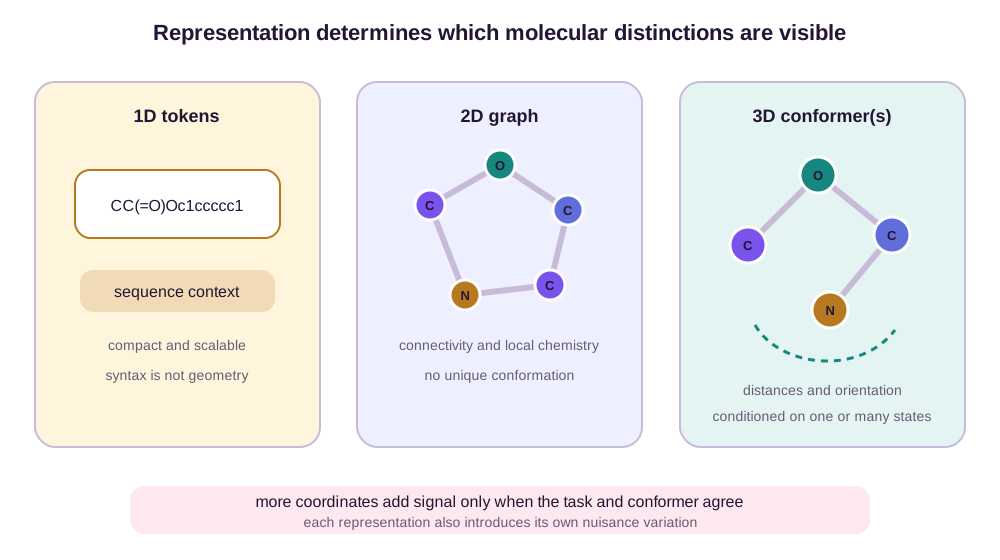
A molecule can be written as a string, drawn as a graph, or placed in three-dimensional space. These are not three file formats for the same information. Each makes some molecular distinctions explicit, hides others, and introduces its own nuisance variation.

That observation changes how a property-prediction result should be read. A sequence model may exploit a huge unlabeled corpus but spend capacity learning notation. A graph model receives connectivity directly but cannot infer which conformation was measured. A geometric model sees coordinates, yet those coordinates may describe only one arbitrary member of a thermal ensemble. More information can help in principle; in finite data, mismatched information can become a shortcut or a source of variance.

The right starting question is therefore not “Which molecular model is best?” It is: What physical object generated the label, what part of that object is observed, and what kind of future molecule should the evaluation imitate?

A representation defines the prediction problem

Let \(M\) denote the complete molecular state relevant to a measurement and let \(R=r(M)\) be the representation supplied to a model. For squared-error prediction, the optimal predictor based on \(R\) is

\[f^\star(R)=\mathbb{E}[Y\mid R].\]

Its irreducible risk is

\[\mathbb{E}\left[(Y-f^\star(R))^2\right] = \mathbb{E}\left[\operatorname{Var}(Y\mid R)\right].\]

This equation is the cleanest way to think about molecular representation. If two physically different states collapse to the same \(R\) but have different labels, no architecture can remove the resulting conditional variance. Conversely, adding coordinates reduces ambiguity only when those coordinates are relevant and reliable.

A collision has a numerical error floor

Consider a flexible molecule \(F\) with one bond graph and two equally populated conformers. Suppose a conformation-specific observable is \(Y=2\) in the folded state and \(Y=8\) in the extended state. A 2D graph representation maps both states to the same value \(R_F\). The best graph-only squared-error predictor is

\[f^\star(R_F) = \frac12(2)+\frac12(8) =5.\]

Its conditional variance is

\[\operatorname{Var}(Y\mid R_F) = \frac12(2-5)^2+ \frac12(8-5)^2 =9.\]

Every graph-only model therefore has conditional mean-squared error at least \(9\) on this population, even with infinite data and perfect optimization. A 3D representation that distinguishes the two conformers can reduce this particular collision to zero if coordinates are exact and the label is truly state-specific. It cannot remove assay noise or uncertainty about which state was measured.

The same calculation applies to an analogue series. Let molecules \(A_1,A_2,A_3\) share a core scaffold and differ by one substituent. A coarse fingerprint that hashes away the distinguishing environment could map \(A_1\) and \(A_2\) to one bin. If their labels differ, the bin average is the Bayes predictor and the within-bin variance is an information loss, not a training failure. A richer representation helps only by separating label-relevant states; adding nuisance detail can increase finite-sample variance without changing the Bayes target.

1D: strings and sequences

SMILES linearizes a molecular graph into tokens (Weininger, 1988). It is compact, ubiquitous, and compatible with the machinery developed for language models. Long-range token dependencies can encode ring closures, branches, stereochemical marks, and recurring chemical fragments.

But SMILES order is not molecular order. The same graph can have many valid traversals and therefore many valid strings. A canonicalizer chooses one, while randomized SMILES presents several equivalent views during training. Canonicalization reduces duplication but creates arbitrary sequential regularities; augmentation encourages invariance but increases training cost. A token model must learn both chemistry and the grammar used to serialize it.

Strings are attractive when data scale and metadata dominate geometry: broad bioactivity corpora, reaction records, patents, assay text, and multi-task pretraining. They are less natural when the label depends sensitively on a particular pose or local force. A valid string also does not guarantee a stable three-dimensional molecule under the conditions of interest.

2D: graphs and fingerprints

A molecular graph represents atoms as nodes and bonds as edges. Node attributes can include element, formal charge, aromaticity, chirality, and hybridization; edge attributes can include bond order and stereochemistry. Message passing respects atom indexing by construction, and a permutation-invariant readout produces a molecular prediction.

The graph makes connectivity explicit, but it still omits a unique geometry. Cis/trans and tetrahedral stereochemistry can be stored as discrete labels, yet a graph does not specify a protein-bound pose, solvent-dependent conformation, or a distribution of torsional states.

Learned graph representations should also be compared with strong fixed descriptors. Extended-connectivity fingerprints record hashed circular atom environments and remain remarkably competitive on many small molecular datasets (Rogers & Hahn, 2010). An ECFP model is fast, stable, and difficult to beat when a target is largely determined by local substructures and labeled data are scarce. Beating a weak neural baseline while omitting fingerprints establishes little.

3D: conformers and atomic environments

A geometric representation supplies atomic coordinates \(X=(x_1,\ldots,x_N)\) in addition to atom types and connectivity. Distances, angles, and torsions become observable. An invariant model predicts a scalar property such as energy or polarizability; an equivariant model can predict vectors such as forces or dipoles. The companion post on scalar and vector geometric graph networks develops this architectural distinction.

The scientific meaning of “the coordinates” depends on the dataset. QM9 provides optimized geometries and quantum-chemical properties for roughly 134,000 small organic molecules (Ramakrishnan et al., 2014). Its labels describe a specified electronic-structure calculation near an equilibrium structure. A solubility or bioactivity measurement, in contrast, reflects temperature, solvent, protonation, experimental protocol, and often many conformers. Giving such a task one inexpensive generated conformer does not turn it into a clean 3D problem.

The same molecule may have many relevant conformers

Suppose a molecular graph has conformers \(X_1,\ldots,X_C\) with free energies \(G_1,\ldots,G_C\). At inverse temperature \(\beta\), an idealized population is

\[\pi_c = \frac{\exp(-\beta G_c)} {\sum_{k=1}^{C}\exp(-\beta G_k)}.\]

For an observable that averages over interconverting states,

\[\overline{Y} \approx \sum_{c=1}^{C}\pi_c\,Y(X_c).\]

The equation exposes two uncertainties. The conformer set may be incomplete, and the weights may be inaccurate because the environment and free energies are approximate. Uniformly averaging conformer embeddings silently assumes equal populations; choosing only the lowest-energy conformer assumes the observable is dominated by that state.

One ensemble reverses a screening decision

Carry molecule \(F\) with three generated conformers. At \(298\) K, use \(RT\approx0.593\) kcal/mol and relative free energies

\[(\Delta G_1,\Delta G_2,\Delta G_3) = (0,0.6,1.2)\ \mathrm{kcal/mol}.\]

The unnormalized Boltzmann weights are

\[\left( 1, e^{-0.6/0.593}, e^{-1.2/0.593} \right) \approx (1,0.364,0.132),\]

which normalize to approximately \((0.668,0.243,0.088)\). Rounding explains why the displayed weights sum to \(0.999\) rather than exactly one.

Suppose the conformation-specific surrogate predicts \(Y(X_c)=(2,8,14)\) and the experimental observable is a linear population average. Then

\[\overline Y_{\mathrm{Boltzmann}} \approx 0.668(2)+0.243(8)+0.088(14) \approx4.51.\]

The lowest-conformer rule predicts \(2\). Uniform averaging predicts \((2+8+14)/3=8\). If a screening rule accepts candidates above \(5\), uniform aggregation accepts \(F\) while both the Boltzmann and lowest-state rules reject it. Against a rigid analogue predicted at \(4.7\), uniform aggregation ranks \(F\) first, whereas the Boltzmann estimate ranks the rigid analogue first. The aggregation rule has changed the experimental action, not merely the third decimal place.

This toy average assumes rapid interconversion, equilibrium populations, a linear observable, and free energies appropriate to the assay environment. Binding, fluorescence, and reaction rates can violate one or more assumptions. A nonlinear assay response generally requires averaging the physical response before applying the reported transformation; averaging log-values can differ from logging an average. The calculation is useful because it states exactly which ensemble claim the number \(4.51\) represents.

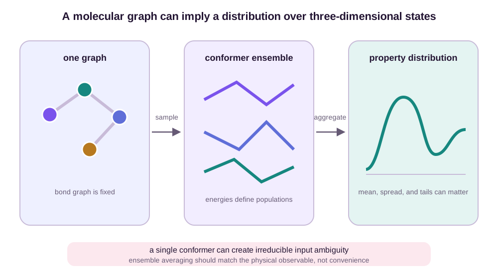
The correct aggregation is task-dependent. A gas-phase quantum property may be evaluated at one optimized geometry. A room-temperature spectrum averages an ensemble. Binding affinity depends on ligand and receptor conformations, protonation, solvent, and the thermodynamic path—not merely on an isolated ligand conformer. A force-field dataset such as MD17 changes the unit of prediction again: each geometry is a separate state with its own energy and forces, not another noisy row for the same molecule.

Conformer generation can still help a 2D deployment setting. A model can pool several predicted conformers, marginalize their predictions, or use 3D data only during pretraining. 3D Infomax, for example, transfers geometric information into a graph encoder that does not require coordinates at inference (Stärk et al., 2022). The important point is to report whether test-time geometry is experimental, computed, generated, or absent.

Task regimes imply different representations

Task	Label-generating object	Natural input	Central ambiguity
Aqueous solubility	Molecule in solvent under an assay protocol	1D/2D plus conditions	Ionization, solid state, and measurement noise
Bioactivity classification	Molecule–target–assay interaction	2D molecule plus target/assay context	Dataset bias, inactive definition, and target shift
QM9 energy or orbital property	Optimized gas-phase geometry and computational method	3D conformer	Limited elements, size, and equilibrium regime
Conformer energy ranking	Several states of one molecular graph	3D conformer ensemble	Missing conformers and energy accuracy
Protein–ligand affinity	Bound complex and thermodynamic environment	3D complex plus conditions	Pose, receptor flexibility, protonation, and entropy
Atomic forces	One instantaneous atomic configuration	3D coordinates	Coverage of off-equilibrium configurations

The table also explains why a single benchmark suite cannot identify a universally superior molecular representation. MoleculeNet was valuable because it standardized diverse datasets, metrics, featurizations, and splits (Wu et al., 2018). Its tasks deliberately span different physical meanings. Averaging ranks across them may summarize engineering breadth, but it does not create one coherent scientific target.

Fidelity and inference-time availability define the task

A label is always conditional on a method or protocol. For the flexible molecule \(F\), three plausible targets are different random variables:

• a DFT energy at one optimized geometry, tied to a functional, basis, charge, and gas-phase state;
• a force-field conformer free energy, tied to a solvent model and parameterization;
• an experimental assay value, tied to temperature, ionization, impurities, and laboratory protocol.

Training them in one column without a fidelity indicator asks the model to average incompatible procedures. A multi-fidelity model can instead condition on the procedure or learn a correction such as

\[Y_{\mathrm{high}}(M) = Y_{\mathrm{low}}(M) + \Delta(M).\]

This decomposition is a modeling choice. It helps when the low-fidelity calculation captures shared trends and paired high-fidelity labels identify the residual. It fails when the two procedures describe different physical states or when \(Y_{\mathrm{low}}\) is unavailable for future candidates.

Inference availability is as important as information content. An experimental crystal structure may predict solubility well but cannot screen an unsynthesized library. A generated conformer is available prospectively, but its errors become part of the pipeline. A DFT geometry may be accurate enough yet cost more than the decision permits. The representation supplied during evaluation must be produced by the same prospective workflow. Otherwise the benchmark measures an oracle-assisted task.

For the analogue series \(A_1,A_2,A_3\), suppose the deployment input is standardized 2D structure and assay conditions. A 3D teacher may improve a 2D student during pretraining, but the final claim remains 2D inference. If evaluation instead gives each test molecule its experimentally resolved bound pose, the estimand has changed to property prediction conditional on a pose. Those are both legitimate tasks; their scores are not directly comparable.

A split defines the generalization claim

A random row split asks whether the model can interpolate among samples drawn from the same mixture. In chemical datasets, this often places close analogues on both sides of the boundary. If a medicinal-chemistry series differs only by one substituent, the test set may be chemically familiar even when its exact molecules are unseen.

A scaffold split groups molecules by a core scaffold and assigns entire groups to one partition. It is a rougher proxy for discovering new chemical families. A temporal split trains on measurements available before a cutoff and tests on later measurements; when timestamps reflect an actual discovery campaign, this is often closest to prospective deployment. Target-family, laboratory, or acquisition-source splits may be more appropriate when those shifts dominate.

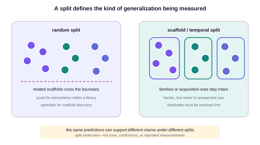
No split is intrinsically honest. It is honest only relative to a deployment claim. Random splits are reasonable when future samples will come from the same enumerated library. Scaffold splits can be unnecessarily pessimistic when optimization deliberately explores close analogues. Temporal splits can be confounded by changes in assay protocol.

Before splitting, the unit of independence must be defined. Common leakage routes include:

• the same molecule under different SMILES strings;
• salts, tautomers, stereoisomers, or protonation states inconsistently standardized;
• multiple conformers of one molecule divided across partitions;
• repeated assay measurements or near-duplicate records;
• pretraining data that contain downstream test molecules or labels;
• protein–ligand complexes sharing nearly identical proteins and ligand series.

Wallach and Heifets showed that redundancy in ligand benchmarks can reward memorization rather than prospective generalization (Wallach & Heifets, 2018). The lesson is broader than virtual screening: similarity across the split must be measured, not assumed from row counts.

Put six related records on opposite sides

The independent unit depends on deployment. Consider this small campaign, where \(A_1,A_2,A_3\) share scaffold \(S\) and \(B_1\) has scaffold \(T\):

Record	Molecule/state	Scaffold	Date	Protocol	Relationship
\(r_1\)	\(A_1\), conformer 1	\(S\)	January	lab P	first measurement
\(r_2\)	\(A_1\), conformer 1	\(S\)	January	lab P	duplicate SMILES and replicate
\(r_3\)	\(A_1\), conformer 2	\(S\)	January	computed Q	same molecule, another state
\(r_4\)	\(A_2\)	\(S\)	February	lab P	one-substituent analogue
\(r_5\)	\(A_3\)	\(S\)	August	lab P2	later analogue, revised assay
\(r_6\)	\(B_1\)	\(T\)	September	lab P2	later new scaffold

A random row split can train on \(r_1\) and test on \(r_2\). The nominal test row is unseen, but the physical molecule, conformation, protocol, and often label noise are shared. This estimates reproducibility or interpolation among records from the same mixture, not performance on a new molecule. Putting \(r_3\) in test is only slightly harder if the model input omits conformer identity: the same graph remains in training.

A molecule split groups \(r_1,r_2,r_3\). Testing on \(A_2\) now estimates performance on a new molecular identity drawn near known chemistry. Dependence remains because \(A_2\) shares scaffold \(S\) and the same medicinal-chemistry program with \(A_1\). This residual similarity may be exactly what analogue optimization expects, so it is not automatically leakage. It does invalidate a claim about unseen chemical families.

A scaffold split keeps all of \(A_1,A_2,A_3\) together and can test on \(B_1\). It estimates transfer to the chosen scaffold equivalence classes, conditional on the rest of the data-generating process. Shared protein targets, assay plates, laboratories, or near-identical side chains can still cross the boundary. The molecular-framework definition introduced by Bemis & Murcko, 1996 is also a crude equivalence relation for splitting: molecules can be highly similar despite different formal scaffolds, or diverse despite sharing one.

A temporal split trains on January–February and tests on August–September. Here it places \(r_5\) and \(r_6\) in test. This resembles prospective arrival, but it mixes two shifts: \(r_5\) is a close later analogue measured with revised protocol P2, whereas \(r_6\) is both later and a new scaffold. Their average loss estimates the actual future mixture only if that mixture resembles August–September. It does not isolate chemical novelty from assay drift.

The estimand can be written explicitly. For loss \(\ell\) and deployment population \(P_{\mathrm{deploy}}\), the intended quantity is

\[\mathcal R_{\mathrm{deploy}}(f) = \mathbb E_{(X,Y)\sim P_{\mathrm{deploy}}} [\ell(f(X),Y)].\]

Each split constructs an empirical proxy using a different rule for which records may be dependent. Reporting the split name without defining the independent unit, equivalence relation, and future population leaves \(P_{\mathrm{deploy}}\) unspecified. The six records make the choice testable: duplicates should be grouped before any split; conformers should be grouped for molecule-level deployment but separated when each geometry is the prediction unit; protocol changes should be stratified or modeled rather than silently interpreted as molecular error.

Pretraining helps when its invariances match deployment

Molecular pretraining can exploit far more unlabeled structures than any one property dataset. The objective, however, decides what transfers.

Masked atom or bond prediction teaches local chemistry but may be solved through easy neighborhood statistics. Graph-level multi-task supervision teaches correlations across assays but inherits their missingness and bias. Contrastive objectives can align randomized strings, graph augmentations, conformers, images, spectra, or assay descriptions. Geometry-aware pretraining can inject 3D correlations into a 2D encoder.

Hu et al. showed that combining node-level and graph-level objectives can improve molecular graph transfer (Hu et al., 2020). The durable principle is not that pretraining always helps. It is that pretraining should expose variations the downstream model must ignore and distinctions it must preserve.

For example, two randomized SMILES of the same molecule are useful positive pairs because traversal order is a nuisance. Two low-energy conformers may be positives for a graph-level identity task, but forcing their embeddings to coincide is questionable if the downstream label is conformer energy. A 3D objective trained only on equilibrium structures may transfer poorly to transition states or strained poses.

Pretraining comparisons should therefore control at least four quantities: architecture, number of unique molecules, label access, and domain overlap. A larger pretrained model may win because it saw more chemistry or even test-set analogues, not because its objective discovered a more general representation.

Positive pairs declare invariance

Let \(z_\theta(v)\) be an embedding of a molecular view \(v\). A contrastive positive pair minimizes a distance such as

\[\lVert z_\theta(v_1)-z_\theta(v_2)\rVert^2.\]

When \(v_1\) and \(v_2\) are randomized SMILES of \(A_1\), the objective declares traversal order irrelevant. That matches any molecular property. When the pair contains conformers 1 and 2 of \(F\), the objective declares their distinction irrelevant. It matches graph identity but conflicts with the conformation-specific labels \(2\) and \(8\) from the collision example. Pretraining has not learned a universally chemical invariance; it has chosen a quotient of the input space.

Overlap can be quantified rather than mentioned vaguely. Suppose a pretraining corpus contains one million structures and a downstream test set contains 200 molecules. An audit finds 30 exact test molecules in pretraining and 90 additional test molecules with fingerprint similarity above \(0.8\) to a pretrained molecule. Then only 80 of 200 test cases lack either form of close exposure under this audit. A reported test average mixes at least three regimes: 15% exact overlap, 45% analogue overlap, and 40% more distant transfer.

Removing the 30 exact molecules fixes only the narrowest leakage. The analogue series \(A_1,A_2,A_3\) may still straddle pretraining and test, allowing the encoder to learn its scaffold and substituent statistics. That exposure is legitimate for a claim about adapting a broad chemical foundation model, but not for a claim that the objective extrapolates to unseen chemistry. Useful reports give performance separately for exact, near, and distant groups and compare against an architecture trained from scratch on the same downstream labels.

Evaluation needs more than one aggregate metric

Regression benchmarks usually report MAE or RMSE. MAE describes a typical absolute miss; RMSE emphasizes large errors. Classification benchmarks often report ROC-AUC, which can remain high under severe class imbalance; precision–recall AUC is more sensitive to performance on a rare active class. These metrics answer different questions and should not be interchanged after looking at results.

Aggregate scores also erase chemical structure. A useful evaluation stratifies error by scaffold novelty, molecular size, charge, element, target family, conformer energy, and distance from the training set. It reports repeated seeds and confidence intervals. For screening or materials discovery, it pays special attention to ranking at the extreme tail, because the top candidates—not the median molecule—drive experiments.

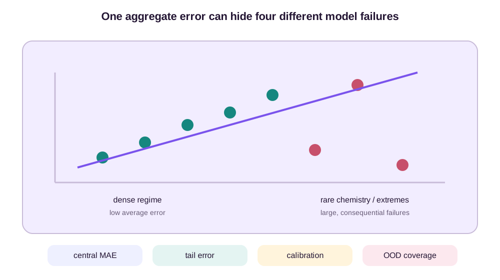
A strong report also includes simple baselines, computational cost, and data efficiency. A deep model that improves MAE by a negligible amount over ECFP plus gradient boosting while requiring thousands of times more compute may still be useful—but its contribution is different from a claim of better representation learning.

One prediction set gives three different verdicts

Take six screening candidates with reference values and predictions

\[\mathbf y=(2,4,6,8,10,12), \qquad \widehat{\mathbf y}=(2,5,5,9,13,7).\]

The residuals are \((0,1,-1,1,3,-5)\), so

\[\mathrm{MAE} = \frac{11}{6} \approx1.83, \qquad \mathrm{RMSE} = \sqrt{\frac{0+1+1+1+9+25}{6}} = \sqrt{\frac{37}{6}} \approx2.48.\]

RMSE is larger because the missed candidate with true value \(12\) contributes squared error \(25\). Whether \(1.83\) is acceptable depends on the action threshold and measurement units.

Suppose the experiment can test two molecules and the true “hits” are the top two reference values, \(10\) and \(12\). Selecting the two largest means chooses predictions \(13\) and \(9\), whose true values are \(10\) and \(8\). Precision among the two selected molecules is \(1/2\). Since two of six molecules are hits, random selection has expected hit fraction \(1/3\); the enrichment factor is

\[\mathrm{EF}_{2} = \frac{1/2}{1/3} =1.5.\]

The same model can therefore have a moderate MAE, a worse RMSE driven by one miss, and only 1.5-fold top-two enrichment. None of the three numbers determines the others. A screening claim should report the metric at the actual experimental budget.

Uncertainty should change a decision

Molecular labels combine at least two kinds of uncertainty. Aleatoric uncertainty comes from measurement noise, uncontrolled conditions, conformer populations, and irreducible ambiguity in the representation. Epistemic uncertainty comes from limited training coverage and model uncertainty. More data from the same regime can reduce the second but not necessarily the first.

Suppose a regressor returns mean \(\mu(x)\) and scale \(\sigma(x)\). Under a Gaussian predictive model, training may use

\[-\log p(y\mid x) = \frac{(y-\mu(x))^2}{2\sigma(x)^2} +\frac{1}{2}\log \sigma(x)^2 +\text{constant}.\]

This objective rewards both accurate means and honest scales. Yet a low negative log-likelihood on an in-distribution test set does not establish calibrated uncertainty under scaffold or temporal shift.

Calibration asks whether intervals behave as advertised. If \(I_{0.9}(x)\) is a predicted 90% interval, empirical coverage should satisfy

\[\frac{1}{n} \sum_{i=1}^{n} \mathbf{1}\{y_i\in I_{0.9}(x_i)\} \approx 0.9.\]

Coverage must be paired with sharpness: an interval spanning the entire label range is well covered but useless. Calibration should also be checked by chemical subgroup and distance to training data. Deep ensembles, evidential heads, Bayesian approximations, and conformal intervals make different assumptions; comparative studies find no single method uniformly reliable across molecular tasks (Hirschfeld et al., 2020).

The operational test is whether uncertainty improves a decision. Can it identify predictions that need a quantum calculation, prioritize experiments with high expected value, or abstain on unsupported chemistry? If not, the uncertainty estimate is decorative.

Continue the six-candidate example with predictive standard deviations

\[\boldsymbol\sigma = (0.5,1,1,1,1.5,4).\]

Approximate 90% Gaussian intervals are \(\widehat y_i\pm1.645\sigma_i\). The first four reference values lie inside their intervals. Candidate five has error \(3\) but half-width \(2.4675\), so it is uncovered. Candidate six has error \(5\) but half-width \(6.58\), so it is covered. Empirical coverage is therefore \(5/6\approx83.3\%\), below the nominal 90% level. The average interval width is

\[\frac{2(1.645)}{6} \sum_i\sigma_i = \frac{3.29}{6}(9) \approx4.94.\]

Six examples cannot establish calibration, but the arithmetic shows why coverage and sharpness must appear together. The broad interval for candidate six repairs coverage while admitting that its mean is unreliable. Among the two high-value references \(10\) and \(12\), coverage is only \(1/2\), revealing worse tail calibration than aggregate coverage.

Uncertainty changes the two-experiment decision. Mean ranking selected candidates five and four, finding only the true value \(10\). An optimistic upper-confidence score \(\widehat y+1.645\sigma\) gives approximately

\[(2.82,6.65,6.65,10.65,15.47,13.58).\]

It selects candidates five and six, whose reference values are the true top two, \(10\) and \(12\). In this toy set, uncertainty-aware acquisition improves top-two precision from \(1/2\) to \(1\). The result is not a general theorem about upper confidence bounds: an overinflated \(\sigma\) can waste the budget, and shift can destroy calibration. It is the correct form of evidence for an uncertainty claim because the estimate changes a specified action and the realized utility is measured.

An abstention policy gives another interpretation. If predictions with \(\sigma>2\) are sent to an expensive quantum calculation, only candidate six is deferred. The cheap model serves five molecules and the high-fidelity method catches the largest mean error. Reporting the retained fraction, error after abstention, and cost of deferral makes the tradeoff visible.

What benchmark accuracy hides

A benchmark score compresses an entire experimental system into one number. It usually hides:

• whether labels are experimental, simulated, or mixtures of protocols;
• whether uncertainty comes from the assay, conformers, or chemical novelty;
• whether the split resembles prospective use;
• how many close analogues occur across partitions;
• whether test-time coordinates are realistic and available;
• whether pretraining overlaps the benchmark domain;
• which chemical subgroups dominate the aggregate metric;
• how prediction cost compares with data acquisition cost.

This is why molecular property prediction should be framed from the outside inward. Define the deployment population and label-generating process. Choose the representation that contains the necessary information at inference time. Split at the unit that will truly be new. Compare against strong, cheap baselines. Report error distributions and calibrated uncertainty, not only their averages.

A property-prediction claim can be checked as one contract:

Contract item	Question	Failure exposed by the running examples
Physical object and label	Which state, ensemble, fidelity, and protocol generated \(Y\)?	DFT conformer energy and experimental ensemble response are mixed
Representation	Which distinctions survive in \(R\) at inference?	Two conformers collide and impose MSE floor \(9\)
Aggregation	How are several states combined?	Lowest, uniform, and Boltzmann rules reverse the screening decision
Independent unit	Which records count as one dependent group?	Replicate \(r_2\) or conformer \(r_3\) crosses a row split
Deployment population	Are future cases new rows, molecules, scaffolds, or times?	Molecule, scaffold, and temporal splits estimate different risks
Pretraining exposure	Which exact or analogous test chemistry was seen?	15% exact and 45% analogue overlap are hidden in one score
Metric and tail budget	Which errors change the experimental shortlist?	MAE \(1.83\) coexists with top-two enrichment \(1.5\)
Uncertainty action	Does uncertainty alter acquisition or abstention?	Upper confidence recovers both top candidates; mean ranking misses one

The contract prevents a narrow architectural result from expanding into a scientific claim. A graph network can be the best predictor of assay rows under a random split without being the best predictor of unseen scaffolds. A 3D model can win with oracle conformers while being unusable before synthesis. A calibrated interval on familiar analogues can fail on a later assay protocol. Each qualifier identifies a different population or available input, not a rhetorical caveat.

The most sophisticated architecture cannot repair a benchmark that asks the wrong question. Conversely, a simple fingerprint or graph model can be scientifically valuable when the representation, split, and decision are aligned. Molecular machine learning progresses when improvements survive that alignment—not merely when another decimal place moves.

References

1. Weininger, D. (1988). SMILES, a Chemical Language and Information System. 1. Introduction to Methodology and Encoding Rules. Journal of Chemical Information and Computer Sciences. ↩
2. Rogers, D., & Hahn, M. (2010). Extended-Connectivity Fingerprints. Journal of Chemical Information and Modeling. ↩
3. Ramakrishnan, R., Dral, P. O., Rupp, M., & von Lilienfeld, O. A. (2014). Quantum Chemistry Structures and Properties of 134 Kilo Molecules. Scientific Data. ↩
4. Wu, Z. et al. (2018). MoleculeNet: A Benchmark for Molecular Machine Learning. Chemical Science. ↩
5. Wallach, I., & Heifets, A. (2018). Most Ligand-Based Classification Benchmarks Reward Memorization Rather Than Generalization. Journal of Chemical Information and Modeling. ↩
6. Bemis, G. W., & Murcko, M. A. (1996). The Properties of Known Drugs. 1. Molecular Frameworks. Journal of Medicinal Chemistry. ↩
7. Hu, W. et al. (2020). Strategies for Pre-Training Graph Neural Networks. ICLR. ↩
8. Stärk, H. et al. (2022). 3D Infomax Improves GNNs for Molecular Property Prediction. ICML. ↩
9. Hirschfeld, L., Swanson, K., Yang, K., Barzilay, R., & Coley, C. W. (2020). Uncertainty Quantification Using Neural Networks for Molecular Property Prediction. Journal of Chemical Information and Modeling. ↩

---

Figure provenance. All four molprop_ diagrams are original SVG illustrations generated by scripts/generate_molprop_figures.py. They synthesize standard representation, splitting, conformer, and evaluation concepts described in the cited primary literature; no third-party artwork is reproduced.