ODEs, SDEs, and Probability Flow

Adapted from my 2025 Machine Learning for Molecules and Geometric Deep Learning lectures. One particle ensemble is carried from a deterministic flow map to a density, a probability current, and two reverse-time samplers; The Fokker–Planck Equation provides the full PDE derivation.

Generative models need a way to move probability. A deterministic model can move every sample along a velocity field. A stochastic model can add random Brownian kicks while it moves. These mechanisms produce different trajectories, but trajectories are not the final object of interest. What matters for generation is the probability distribution reached at each time.

The distinction between trajectories and distributions leads to a useful equivalence. A diffusion process has a deterministic probability-flow ODE whose marginal density matches the diffusion at every time. The reverse-time diffusion and the reverse probability flow can therefore start from the same noise distribution and arrive at the same data distribution, even though one produces noisy paths and the other produces smooth paths.

The score \(\nabla_{\mathbf{x}}\log p_t(\mathbf{x})\) makes this equivalence possible. It measures how the current density varies in space. In the reverse SDE, the score compensates for diffusion while time runs backward. In the probability-flow ODE, half of the same correction converts diffusive spreading into deterministic transport.

One Gaussian ensemble will make every step testable. Throughout the post, the initial state is

\[X_0\sim\mathcal N(2,1).\]

The mean 2 keeps the formulas from hiding behind zero symmetry, while unit initial variance makes the numerical checks simple. The deterministic sections first allow a general scale factor. The stochastic sections then choose unit Brownian noise, for which the variance grows from 1 to \(1+t\). At the final time \(T=3\), the distribution is \(\mathcal N(2,4)\).

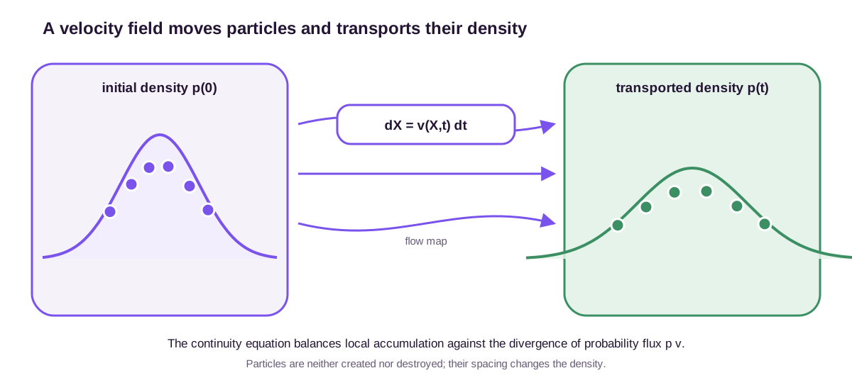
An ODE transports particles through a flow map

Let \(\mathbf{X}_t\in\mathbb{R}^{d}\) follow the ordinary differential equation

\[d\mathbf{X}_t =\mathbf{v}(\mathbf{X}_t,t)\,dt.\]

The vector field \(\mathbf{v}:\mathbb{R}^{d}\times[0,T]\to\mathbb{R}^{d}\) assigns a velocity to every position and time. Under standard regularity conditions, each initial point \(\mathbf{X}_0=\mathbf{x}_0\) determines one trajectory. We write the resulting flow map as

\[\boldsymbol{\psi}_t(\mathbf{x}_0)=\mathbf{X}_t.\]

If the initial state is random, \(\mathbf{X}_0\sim p_0\), the same map pushes the entire distribution forward:

\[p_t=(\boldsymbol{\psi}_t)_{\#}p_0.\]

The pushforward notation says that a sample drawn from \(p_0\) and transformed by \(\boldsymbol{\psi}_t\) has density \(p_t\). The ODE operates on particles, while the pushforward describes their ensemble. This statement assumes that the ODE has a unique solution over the interval of interest. A locally Lipschitz velocity is a standard sufficient condition; exploding trajectories or nonunique solutions require additional care.

Translation changes location but not volume

A constant velocity gives the simplest example. In one dimension, let

\[dX_t=c\,dt, \qquad X_0\sim p_0.\]

The solution is \(X_t=X_0+ct\), so the density is translated without changing shape:

\[p_t(x)=p_0(x-ct).\]

The particle equation and density equation contain the same information in different forms. Differentiating the translated density gives

\[\frac{\partial p_t(x)}{\partial t} =-c\frac{\partial p_t(x)}{\partial x} =-\frac{\partial}{\partial x}\bigl(c\,p_t(x)\bigr).\]

For a general vector field, this becomes the continuity equation:

\[\frac{\partial p_t(\mathbf{x})}{\partial t} =-\nabla_{\mathbf{x}}\cdot \bigl[p_t(\mathbf{x})\mathbf{v}(\mathbf{x},t)\bigr].\]

The product \(p_t\mathbf{v}\) is probability flux. Its divergence measures net outflow from a small region. Positive divergence depletes density; negative divergence accumulates it.

An affine flow changes the Gaussian volume

Translation does not exercise the Jacobian of the flow map. For the running Gaussian, consider instead

\[\frac{dX_t}{dt}=\alpha(t)(X_t-2),\]

where \(\alpha(t)\) is a prescribed scalar rate. Subtracting the fixed center and integrating gives

\[X_t-2=a_t(X_0-2), \qquad a_t=\exp\!\left(\int_0^t\alpha(r)\,dr\right)>0.\]

Thus the flow map is \(\psi_t(x_0)=2+a_t(x_0-2)\). Its one-dimensional Jacobian is \(\partial\psi_t/\partial x_0=a_t\). Conservation of probability in a small interval requires

\[p_t(x)\,dx=p_0(x_0)\,dx_0, \qquad x_0=2+\frac{x-2}{a_t}.\]

Since \(dx=a_t\,dx_0\), the pushed-forward density is

\[p_t(x) =\frac{1}{a_t} p_0\!\left(2+\frac{x-2}{a_t}\right).\]

For \(X_0\sim\mathcal N(2,1)\), this density is \(\mathcal N(2,a_t^2)\). Every deviation from the mean is multiplied by \(a_t\), so the variance is multiplied by \(a_t^2\). The density height falls by \(1/a_t\) because the same probability mass occupies an interval that is \(a_t\) times wider.

The continuity equation verifies the same result locally. The velocity derivative is \(\partial_x v=\alpha(t)\). Along a trajectory,

\[\begin{aligned} \frac{d}{dt}\log p_t(X_t) &=\partial_t\log p_t(X_t) +v(X_t,t)\,\partial_x\log p_t(X_t)\\ &=-\partial_x v(X_t,t)\\ &=-\alpha(t). \end{aligned}\]

Integrating gives \(\log p_t(X_t)=\log p_0(X_0)-\log a_t\), exactly the Jacobian formula above. The particle map, density pushforward, continuity equation, and log-density change are four descriptions of the same deterministic transport.

Neural ODEs learn the velocity field

A neural ODE parameterizes the vector field with a network \(\mathbf{v}_{\theta}\) (Chen et al., 2018):

\[d\mathbf{X}_t =\mathbf{v}_{\theta}(\mathbf{X}_t,t)\,dt.\]

Numerical integration replaces a fixed sequence of residual blocks with evaluations of a continuous-time vector field. When the ODE is used as a continuous normalizing flow, we also need the density change along each trajectory.

The network is a learned parameter choice, while the change-of-density identity below is exact for the resulting vector field when the ODE solution exists. These two statements should not be conflated: a neural vector field can be represented poorly, and a well-represented field can still be integrated poorly.

Apply the chain rule to \(\log p_t(\mathbf{X}_t)\) and substitute the continuity equation:

\[\begin{aligned} \frac{d}{dt}\log p_t(\mathbf{X}_t) &=\frac{\partial}{\partial t}\log p_t(\mathbf{X}_t) +\mathbf{v}(\mathbf{X}_t,t)^{\mathsf T} \nabla\log p_t(\mathbf{X}_t)\\ &=-\nabla\cdot\mathbf{v}(\mathbf{X}_t,t). \end{aligned}\]

The terms involving \(\mathbf{v}^{\mathsf T}\nabla\log p_t\) cancel. Density decreases along a trajectory when the local flow expands and increases when it contracts. Integrating this scalar equation gives an exact change-of-variables formula:

\[\log p_T(\mathbf{X}_T) =\log p_0(\mathbf{X}_0) -\int_0^T \nabla\cdot\mathbf{v}(\mathbf{X}_t,t)\,dt.\]

This formula is one reason deterministic probability flows are useful: the same ODE solver can transport samples and accumulate likelihoods.

The Jacobian and CNF calculations agree point by point

The affine Gaussian flow provides a complete continuous-normalizing-flow calculation. Choose

\[a_t=\sqrt{1+t}, \qquad \alpha(t)=\frac{d}{dt}\log a_t=\frac{1}{2(1+t)}.\]

At \(T=3\), the map is \(X_3=2+2(X_0-2)\) and its Jacobian determinant is 2. For the particular initial particle \(X_0=3\), the final location is \(X_3=4\). Direct change of variables gives

\[\log p_3(4) =\log p_0(3)-\log 2.\]

The continuous normalizing flow (CNF) calculation accumulates the divergence instead. In one dimension, \(\nabla\cdot v=\partial_xv=1/[2(1+t)]\), so

\[\int_0^3\nabla\cdot v\,dt =\frac12\int_0^3\frac{dt}{1+t} =\frac12\log4 =\log2.\]

Substituting into the instantaneous change-of-variables formula gives the same \(-\log2\) density correction. Numerically,

\[p_0(3)=\frac{e^{-1/2}}{\sqrt{2\pi}}\approx0.2420, \qquad p_3(4)\approx0.1210.\]

The density halves because the flow doubles every local interval. This calculation will reappear after the stochastic derivation: unit Brownian diffusion produces the same Gaussian variance \(1+t\), and its probability-flow ODE turns out to use this exact affine velocity.

Numerical integration adds a separate approximation

The exact ODE defines a flow independently of the solver. Forward Euler with step size \(h\) replaces the flow over one step by

\[X_{t+h}\approx X_t+h\,v_\theta(X_t,t).\]

The approximation error depends on step size and vector-field regularity. An adaptive solver controls a local error estimate, but its tolerance does not certify that \(v_\theta\) represents the desired population velocity. Conversely, an exact population velocity does not prevent endpoint bias if it is integrated with coarse steps. Likelihood computation adds another numerical object, the divergence integral, which must be evaluated consistently along the same approximate trajectory.

An SDE adds randomness at order square root of time

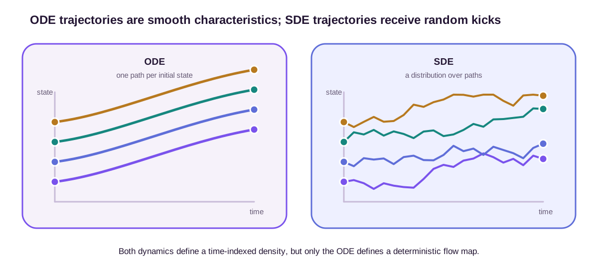
A stochastic differential equation adds a Brownian increment:

\[d\mathbf{X}_t =\mathbf{f}(\mathbf{X}_t,t)\,dt +g(t)\,d\mathbf{W}_t.\]

Here \(\mathbf{f}\) is the drift, \(g(t)\geq 0\) is a scalar diffusion coefficient, and \(\mathbf{W}_t\) is standard \(d\)-dimensional Brownian motion. We restrict attention to isotropic, state-independent diffusion because it exposes the probability-flow identity without extra matrix-divergence terms.

Over a small step \(\Delta t\), Euler–Maruyama gives

\[\mathbf{X}_{t+\Delta t} \approx \mathbf{X}_t +\mathbf{f}(\mathbf{X}_t,t)\Delta t +g(t)\sqrt{\Delta t}\,\boldsymbol{\epsilon}, \qquad \boldsymbol{\epsilon}\sim\mathcal{N}(\mathbf{0},\mathbf{I}).\]

The deterministic displacement is order \(\Delta t\), while the random displacement is order \(\sqrt{\Delta t}\). Brownian paths are continuous but nowhere differentiable, so the SDE does not define an ordinary velocity along each realization.

Conditioned on the current state, the increment has leading-order moments

\[\mathbb E[\mathbf X_{t+\Delta t}-\mathbf X_t\mid\mathbf X_t] =\mathbf f(\mathbf X_t,t)\Delta t,\] \[\operatorname{Cov}(\mathbf X_{t+\Delta t}-\mathbf X_t\mid\mathbf X_t) =g^2(t)\Delta t\,\mathbf I.\]

The drift controls the first conditional moment, while diffusion controls the second. These are local transition-kernel statements, not claims about a realized derivative. For pure Brownian motion with constant \(g\), the Gaussian step is exact; for nonlinear drift, Euler–Maruyama approximates the true transition kernel.

For a scalar unit Brownian step with \(\Delta t=0.01\), the noise has standard deviation \(\sqrt{0.01}=0.1\) and variance 0.01. One hundred independent increments cover one unit of time. Their variances add, so the accumulated noise has variance \(100\times0.01=1\), not 0.01 and not 100. Halving the step makes each kick smaller but doubles the number of kicks; the total variance over a fixed interval stays unchanged.

The running example sets \(f=0\) and \(g=1\):

\[dX_t=dW_t, \qquad X_0\sim\mathcal N(2,1).\]

Brownian increments are independent of the initial state, so \(X_t=X_0+W_t\). Means and variances add:

\[\mathbb E[X_t]=2, \qquad \operatorname{Var}(X_t)=1+t.\]

At \(t=3\), the process reaches \(\mathcal N(2,4)\). An Euler–Maruyama simulation with 300 steps of size 0.01 adds total variance 3 in expectation. The statement concerns the ensemble; one finite batch has a sample variance that fluctuates around 4.

The absence of a deterministic flow map does not prevent us from tracking the density. The density follows a partial differential equation rather than an ODE.

The Fokker–Planck equation exposes probability flux

Let \(p_t(\mathbf{x})\) be the density of the SDE above. Its Fokker–Planck equation is

\[\frac{\partial p_t}{\partial t} =-\nabla\cdot(\mathbf{f}p_t) +\frac{g^2(t)}{2}\Delta p_t.\]

The first term transports density with the drift. The second smooths density through diffusion. The separate post on the Fokker–Planck equation derives both terms from a transition-kernel expansion and from Itô calculus. Repeating those proofs would obscure the bridge needed here. We use the PDE as an identity and perform one algebraic rewrite from density change to current.

Define the score of the marginal density as

\[\mathbf{s}_t(\mathbf{x}) =\nabla_{\mathbf{x}}\log p_t(\mathbf{x}).\]

Since \(\nabla p_t=p_t\nabla\log p_t\), the diffusion term can be written as a divergence:

\[\frac{g^2}{2}\Delta p_t =-\nabla\cdot\left[ -\frac{g^2}{2}\mathbf{s}_t p_t \right].\]

The full Fokker–Planck equation therefore becomes a continuity equation:

\[\frac{\partial p_t}{\partial t} =-\nabla\cdot\left[ p_t\left( \mathbf{f}-\frac{g^2}{2}\mathbf{s}_t \right) \right].\]

The bracketed quantity is the probability current

\[\mathbf{J}_t =p_t\mathbf{f}-\frac{g^2}{2}\nabla p_t,\]

and the density equation is simply \(\partial_t p_t=-\nabla\cdot\mathbf{J}_t\). Dividing current by density gives an effective velocity. The equation no longer displays an explicit Laplacian because diffusive spreading has been absorbed into that density-dependent velocity.

The Gaussian score converts smoothing into outward current

For the running Brownian family,

\[p_t(x) =\frac{1}{\sqrt{2\pi(1+t)}} \exp\!\left[-\frac{(x-2)^2}{2(1+t)}\right].\]

Differentiating its log-density gives

\[s_t(x)=\partial_x\log p_t(x) =-\frac{x-2}{1+t}.\]

The score points toward the mean: it is negative to the right of 2 and positive to the left. Pure diffusion nevertheless moves probability outward. With \(f=0\) and \(g=1\), the probability current is

\[J_t(x) =-\frac12\,\partial_xp_t(x) =\frac{x-2}{2(1+t)}p_t(x).\]

At \(t=3\) and \(x=4\), the score is \(-1/2\), while the current per unit density is

\[\frac{J_3(4)}{p_3(4)}=\frac14.\]

The signs are not contradictory. The score points uphill in density, whereas the diffusive current points downhill in density. The minus sign in \(J=-\frac12p s\) reverses the direction, and the factor \(1/2\) comes from Brownian variance growth.

The current, rather than the score, is the primary globally meaningful object. The identity \(\nabla p=p\nabla\log p\) holds where \(p>0\). At a zero of the density, \(\log p\) and \(J/p\) need not exist even when \(J\) remains finite. A nondegenerate diffusion often makes \(p_t\) smooth and positive for \(t>0\) under standard regularity conditions, but a data distribution at \(t=0\) may be singular or concentrated near a lower-dimensional set. Practical reverse solvers often stop at a small positive time or regularize the endpoint for this reason.

The probability-flow ODE matches the SDE marginals

The continuity form identifies a deterministic vector field:

\[\mathbf{v}_{\mathrm{pf}}(\mathbf{x},t) =\mathbf{f}(\mathbf{x},t) -\frac{g^2(t)}{2} \nabla_{\mathbf{x}}\log p_t(\mathbf{x}).\]

The corresponding probability-flow ODE is

\[d\mathbf{Z}_t =\mathbf{v}_{\mathrm{pf}}(\mathbf{Z}_t,t)\,dt.\]

If \(\mathbf{Z}_0\) and \(\mathbf{X}_0\) have the same distribution, the ODE and SDE have the same marginal density at every time (Song et al., 2021). The claim concerns one-time marginals:

\[\mathbf{Z}_t\overset{d}{=}\mathbf{X}_t \qquad\text{for each }t.\]

The equality is obtained because substituting \(\mathbf v_{\mathrm{pf}}\) into the continuity equation reproduces the Fokker–Planck equation. It is exact under the assumed scalar, state-independent diffusion and sufficient regularity. A state-dependent or matrix-valued diffusion introduces additional divergence terms, so the displayed velocity cannot be copied unchanged.

Five different equality claims

The marginal identity is strong enough for generation and weak enough to permit completely different dynamics. The possible claims should be separated rather than treated as synonyms.

• Endpoint equality requires only \(Z_T\overset d=X_T\). Intermediate distributions may differ.
• One-time marginal equality requires \(Z_t\overset d=X_t\) for every fixed \(t\). This is the probability-flow guarantee.
• Transition-kernel equality requires the conditional laws from one time to another to match. For Markov processes, equal transition kernels together with the same initial law determine all finite-dimensional joint laws.
• Finite-dimensional joint-law equality requires \((Z_{t_1},\ldots,Z_{t_k})\) and \((X_{t_1},\ldots,X_{t_k})\) to match for every finite collection of times. On the canonical continuous-path space, equality of all such laws determines the path measure.
• Path-measure equality packages equality of the full trajectory distributions. Pathwise equality under a specified coupling is stronger: it asks the two realized trajectories to coincide almost surely, not only to have the same law.

The running Gaussian gives explicit witnesses for every failed strengthening. For Brownian diffusion and \(0\le s<t\),

\[X_t\mid X_s=x \sim\mathcal N(x,t-s).\]

The conditional variance is \(t-s>0\). The probability-flow ODE is deterministic, so \(Z_t\mid Z_s=z\) is a point mass at the flow-map image of \(z\). Its conditional variance is zero. The transition kernels cannot agree.

The two-time covariances also differ. Brownian diffusion gives

\[\operatorname{Cov}(X_s,X_t)=\operatorname{Var}(X_s)=1+s,\]

because the future increment \(W_t-W_s\) is independent of \(X_s\). The deterministic Gaussian flow will be derived below as \(Z_t-2=\sqrt{1+t}(Z_0-2)\), which gives

\[\operatorname{Cov}(Z_s,Z_t)=\sqrt{(1+s)(1+t)}.\]

At \(s=1\) and \(t=3\), the Brownian covariance is 2, while the ODE covariance is \(\sqrt8\approx2.828\). Both processes still have marginal variances 2 and 4 at those times.

Quadratic variation separates the path laws without inspecting any density. For a partition \(0=t_0<\cdots<t_n=T\), define

\[[X]_T =\lim_{\max\Delta t_k\to0} \sum_{k=0}^{n-1}(X_{t_{k+1}}-X_{t_k})^2.\]

Unit Brownian diffusion has \([X]_T=T\) almost surely; the smooth probability-flow trajectory has \([Z]_T=0\). At \(T=3\), the values are 3 and 0. Their one-time marginals match, but their path measures are not the same. The companion post on path measures and generative models develops the framework for comparing those full trajectory distributions.

Probability-flow velocity belongs to the ensemble

The probability-flow vector field is an ensemble-level object. Two initial distributions evolved under the same drift and diffusion generally have different scores, so they induce different probability-flow ODEs. We cannot construct the ODE from \(\mathbf{f}\) and \(g\) alone; we also need the current marginal density or its score.

For example, pure unit Brownian motion started from \(\mathcal N(m,s_0^2)\) has

\[v_{\mathrm{pf}}(x,t) =\frac{x-m}{2(s_0^2+t)}.\]

Changing \(m\) or \(s_0^2\) changes the deterministic velocity even though the particle-level SDE \(dX_t=dW_t\) is unchanged. Brownian mechanics alone does not select the probability-flow ODE; Brownian mechanics plus the current ensemble does.

The continuity velocity is also not unique in more than one dimension. A density evolution fixes only \(\nabla\cdot(p\mathbf v)\). If a field \(\mathbf u\) satisfies

\[\nabla\cdot(p_t\mathbf u_t)=0,\]

then \(\mathbf v+\mathbf u\) produces the same density evolution. For a radially symmetric two-dimensional Gaussian, \(\mathbf u(x_1,x_2)=\omega(-x_2,x_1)\) circulates particles around the origin. It has zero divergence, lies tangent to density contours, and therefore satisfies \(\nabla\cdot(p\mathbf u)=0\). The trajectories change while every marginal stays fixed.

The displayed probability-flow velocity is the current divided by density for the Fokker–Planck current chosen above. It is a natural and useful representative, not a proof that only one deterministic flow can realize the same marginal curve. In one dimension with vanishing boundary flux, the current is fixed up to a spatial constant that the boundary condition removes; the higher-dimensional freedom is larger.

The factor \(1/2\) follows directly from the Fokker–Planck diffusion coefficient. Losing it is a common mistake: the reverse-time SDE uses a full \(g^2\mathbf{s}_t\) correction, while the probability-flow ODE uses half.

Reversing a diffusion requires the score

Suppose the forward SDE gradually converts data at time \(0\) into a simple noise distribution at time \(T\). Sampling requires dynamics that run from \(T\) back to \(0\). Reversing only the drift is not enough because Brownian increments are not differentiable paths that can be played backward.

Derive the sign in an increasing reverse clock

Define a new increasing clock \(\tau=T-t\) and the reverse process \(\mathbf{Y}_{\tau}=\mathbf{X}_{T-\tau}\). Its density is \(q_{\tau}=p_{T-\tau}\). The chain rule reverses the density derivative:

\[\partial_\tau q_\tau =-\left.\partial_t p_t\right|_{t=T-\tau}.\]

For compact notation, evaluate every forward coefficient below at \(t=T-\tau\). Negating the forward Fokker–Planck equation gives

\[\partial_\tau q =\nabla\cdot(\mathbf f q) -\frac{g^2}{2}\Delta q.\]

The reverse process adds Brownian noise as \(\tau\) increases, so suppose its drift is \(\mathbf b\). Its own Fokker–Planck equation is

\[\partial_\tau q =-\nabla\cdot(\mathbf b q) +\frac{g^2}{2}\Delta q.\]

Equating the density derivatives and using \(\nabla q=q\nabla\log q\) identifies the standard reverse drift

\[\mathbf b =-\mathbf f+g^2\nabla\log q.\]

Under the regularity assumptions for diffusion time reversal, the resulting reverse-time diffusion is (Anderson, 1982)

\[d\mathbf{Y}_{\tau} =\left[ -\mathbf{f}(\mathbf{Y}_{\tau},T-\tau) +g^2(T-\tau)\nabla\log p_{T-\tau}(\mathbf{Y}_{\tau}) \right]d\tau +g(T-\tau)d\overline{\mathbf{W}}_{\tau}.\]

The first term reverses the forward drift. The score term points toward regions of larger forward marginal density and compensates for the new Brownian noise added during reverse simulation.

The density calculation identifies the required probability flux. As in the previous section, adding a weighted divergence-free current would leave the marginal PDE unchanged, but it would not generally recover the conditional law of the original forward diffusion. The standard reverse drift is the one that reverses the forward process under the stated diffusion assumptions.

Translate once to decreasing forward time

The same formula is often written using the original time variable integrated from \(T\) down to \(0\):

\[d\mathbf{X}_t =\left[ \mathbf{f}(\mathbf{X}_t,t) -g^2(t)\nabla\log p_t(\mathbf{X}_t) \right]dt +g(t)d\overline{\mathbf{W}}_t, \qquad dt<0.\]

The notation \(d\overline{\mathbf W}_t\) in this decreasing-clock display is shorthand for reverse-time Brownian increments whose covariance is \(\lvert dt\rvert\mathbf I\). One should not take a square root of a negative \(dt\). An implementation steps from \(t\) to \(t-h\) with \(h>0\):

\[\mathbf X_{t-h} \approx\mathbf X_t -\left[\mathbf f(\mathbf X_t,t)-g^2(t)\mathbf s_t(\mathbf X_t)\right]h +g(t)\sqrt h\,\boldsymbol\epsilon, \qquad \boldsymbol\epsilon\sim\mathcal N(\mathbf0,\mathbf I).\]

In increasing \(\tau\), the drift is \(-\mathbf f+g^2\mathbf s\). In decreasing \(t\), the bracket is \(\mathbf f-g^2\mathbf s\), but the negative step \(-h\) reverses its effect.

The probability-flow ODE can also be integrated backward. In the increasing reverse clock, its drift is

\[-\mathbf{v}_{\mathrm{pf}}(\mathbf{y},T-\tau) =-\mathbf{f}(\mathbf{y},T-\tau) +\frac{g^2(T-\tau)}{2} \nabla\log p_{T-\tau}(\mathbf{y}).\]

In decreasing \(t\), the deterministic update is correspondingly

\[\mathbf Z_{t-h} \approx\mathbf Z_t -\left[\mathbf f(\mathbf Z_t,t) -\frac{g^2(t)}{2}\mathbf s_t(\mathbf Z_t)\right]h.\]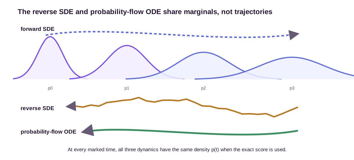

The reverse SDE uses twice the score correction of the reverse ODE because it also injects diffusion. Its stronger inward drift must offset that extra spreading. The deterministic ODE needs only the weaker drift that reproduces the same net probability flux. The Gaussian moment calculation in the next section verifies that explanation numerically.

A Gaussian example makes the factor of two visible

Consider one-dimensional variance-exploding diffusion with constant noise scale:

\[dX_t=\sigma\,dW_t, \qquad X_0\sim\mathcal{N}(m,s_0^2), \qquad s_0>0.\]

Brownian increments are Gaussian, so

\[p_t(x) =\mathcal{N}\!\left(x;m,s_0^2+\sigma^2t\right).\]

The score is

\[\nabla_x\log p_t(x) =-\frac{x-m}{s_0^2+\sigma^2t}.\]

The forward SDE has zero drift. Its probability-flow ODE is therefore

\[\frac{dZ_t}{dt} =\frac{\sigma^2}{2(s_0^2+\sigma^2t)}(Z_t-m).\]

This linear equation has the exact solution

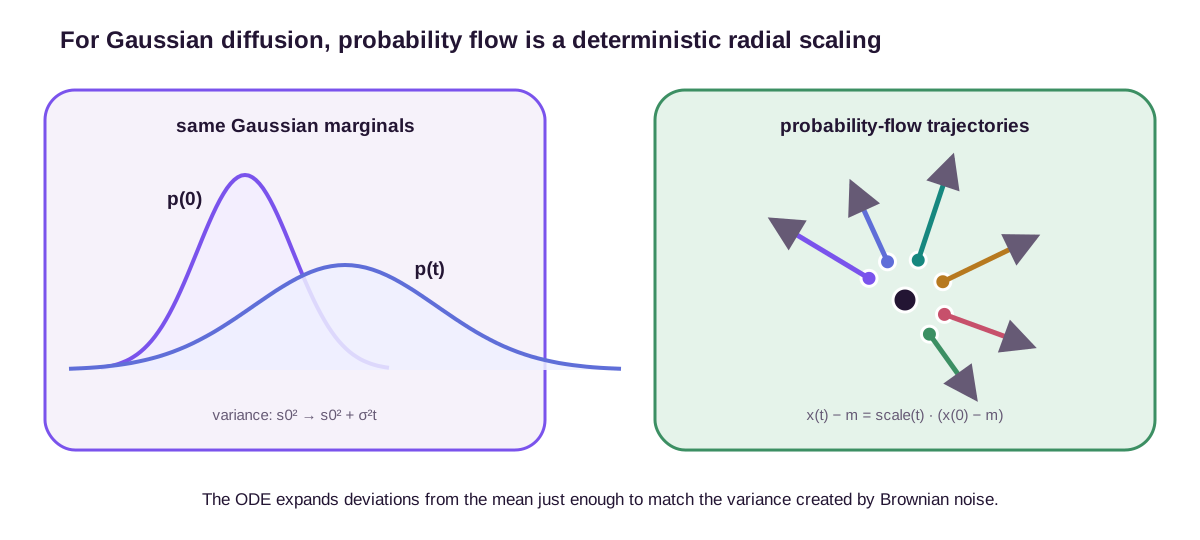
\[Z_t-m =\sqrt{\frac{s_0^2+\sigma^2t}{s_0^2}} (Z_0-m).\]

The flow leaves the mean fixed and scales every deviation by the ratio of standard deviations. If \(Z_0\sim\mathcal{N}(m,s_0^2)\), then \(Z_t\sim\mathcal{N}(m,s_0^2+\sigma^2t)\), exactly matching the SDE.

This solution follows by separating variables rather than guessing a scaling map:

\[\frac{d(Z_t-m)}{Z_t-m} =\frac{\sigma^2\,dt}{2(s_0^2+\sigma^2t)}.\]

Integrating from 0 to \(t\) gives

\[\log\frac{Z_t-m}{Z_0-m} =\frac12\log\frac{s_0^2+\sigma^2t}{s_0^2},\]

which yields the square-root scale above. The probability-flow ODE expands by the ratio of standard deviations, not by the ratio of variances.

For the running values \(m=2\), \(s_0^2=1\), \(\sigma=1\), and \(T=3\),

\[Z_3-2=2(Z_0-2).\]

A particle at \(Z_0=3\) reaches \(Z_3=4\). This is the same affine flow used for the earlier Jacobian and CNF calculation. Brownian diffusion and deterministic scaling both produce \(\mathcal N(2,4)\), but the covariance and quadratic-variation witnesses showed that they do not produce the same process.

Reverse mean and variance expose the factor of two

In the increasing reverse clock, the general reverse SDE drift is

\[-\frac{\sigma^2}{s_0^2+\sigma^2(T-\tau)}(Y_{\tau}-m),\]

while the reverse probability-flow drift is half as large. Both contract the distribution toward \(m\). The running example makes the balance explicit. Its reverse marginal is \(q_\tau=\mathcal N(2,4-\tau)\), so

\[dY_\tau =-\frac{Y_\tau-2}{4-\tau}\,d\tau +d\overline W_\tau.\]

Let \(\mu_\tau=\mathbb E[Y_\tau]\) and \(V_\tau=\operatorname{Var}(Y_\tau)\). The linear SDE gives

\[\frac{d\mu_\tau}{d\tau} =-\frac{\mu_\tau-2}{4-\tau}, \qquad \frac{dV_\tau}{d\tau} =-\frac{2V_\tau}{4-\tau}+1.\]

Starting from \(\mu_0=2\) and \(V_0=4\), substitute \(\mu_\tau=2\) and \(V_\tau=4-\tau\):

\[-\frac{2(4-\tau)}{4-\tau}+1=-1 =\frac{d}{d\tau}(4-\tau).\]

The full score drift contributes \(-2\) to the variance rate, while fresh Brownian noise contributes \(+1\). Their net rate is \(-1\).

The reverse probability-flow ODE has half the drift and no Brownian term:

\[\frac{dZ_\tau}{d\tau} =-\frac{Z_\tau-2}{2(4-\tau)}.\]

Its variance obeys

\[\frac{dV_\tau}{d\tau} =-\frac{V_\tau}{4-\tau}=-1\]

when \(V_\tau=4-\tau\). Half the inward coefficient is enough because the ODE has no outward diffusion to cancel. The mean stays at 2 for both mechanisms.

At \(\tau=3\), both reverse samplers return variance 1. The SDE reaches that variance through inward drift plus noise; the ODE reaches it through a deterministic contraction by \(1/2\). Equality of the final variance is an endpoint statement, and equality of \(4-\tau\) for every \(\tau\) is a marginal statement. Neither repairs their unequal conditional kernels or path laws.

A neural score turns the identities into models

The exact score is unknown because the intermediate marginal \(p_t\) is unknown. Score-based generative models replace it with a neural estimate

\[\mathbf{s}_{\theta}(\mathbf{x},t) \approx\nabla_{\mathbf{x}}\log p_t(\mathbf{x}).\]

The same score network can be inserted into either reverse dynamic:

\[\text{reverse SDE:} \qquad \mathbf{f}-g^2\mathbf{s}_{\theta},\] \[\text{probability-flow ODE:} \qquad \mathbf{f}-\frac{g^2}{2}\mathbf{s}_{\theta},\]

where both expressions use the original time variable integrated backward. Training the score and choosing the forward noise schedule are the subjects of diffusion modeling rather than stochastic calculus; they are developed in the next chapter of the reading path.

More precisely, those expressions define an interface between a learned function and a numerical sampler. The forward schedule supplies \(\mathbf f\) and \(g\). The network supplies an estimate of the score of the particular forward ensemble generated by that schedule and data distribution. The sampler combines them into a reverse drift. Exact reversal additionally assumes that the initial noise sample at \(T\) comes from the true forward marginal \(p_T\).

Three approximations can therefore produce three different endpoint errors.

1. The chosen terminal prior may only approximate \(p_T\).
2. The neural score may differ from \(\nabla\log p_t\) between data and noise.
3. The numerical method may not integrate the learned reverse dynamic accurately.

These errors do not cancel by virtue of the exact probability-flow identity. That identity refers to the exact score, exact terminal marginal, and exact continuous-time dynamics.

A ten-percent score error changes the target variance

The Gaussian family quantifies model error without numerical error. Suppose the probability-flow sampler uses a score with a constant relative bias

\[s_\theta(x,t) =(1+\delta)s_t(x),\]

and suppose we solve the resulting ODE exactly from \(t=3\) down to 0. For the running example, the decreasing-time ODE is

\[\frac{dZ_t}{dt} =\frac{1+\delta}{2(1+t)}(Z_t-2).\]

Integrating backward gives

\[Z_0-2 =4^{-(1+\delta)/2}(Z_3-2).\]

Since the initial noise state has variance 4, the generated endpoint variance is

\[\operatorname{Var}(Z_0) =4\left(4^{-(1+\delta)/2}\right)^2 =4^{-\delta}.\]

The exact score corresponds to \(\delta=0\) and returns variance 1. A ten-percent overestimate, \(\delta=0.1\), returns variance

\[4^{-0.1}\approx0.871.\]

An exact ODE solver cannot remove this 13 percent variance deficit because the solver is accurately integrating the wrong vector field. The reverse SDE responds differently to the same score error because its Brownian term continues to contribute variance; marginal equivalence between the two learned samplers is no longer guaranteed.

A coarse solver creates error even with the exact score

Now set \(\delta=0\) and keep the exact score, but integrate the reverse probability-flow ODE with three Euler steps of size \(h=1\). For a deviation \(D_t=Z_t-2\), the decreasing-time update is

\[D_{t-1} =\left(1-\frac{1}{2(1+t)}\right)D_t.\]

Starting from \(Z_3=4\), so \(D_3=2\), the three multipliers are \(7/8\), \(5/6\), and \(3/4\). Their product is

\[\frac78\cdot\frac56\cdot\frac34 =\frac{35}{64} \approx0.547.\]

Euler therefore returns \(Z_0=2+2(35/64)=3.09375\). The exact contraction is \(1/2\) and returns \(Z_0=3\). The 0.09375 position error is purely numerical. Reducing the step or using a higher-order method attacks this error but does not address the biased-score example above.

For an SDE solver, “accurate” needs a specified sense. Strong error compares approximate and exact paths under a shared Brownian realization. Weak error compares expectations or endpoint distributions. Generation usually emphasizes weak accuracy, while path-dependent observables require more. An ODE solver has no Brownian discretization, but adaptive tolerances can cause different numbers of network evaluations across samples.

Likelihood belongs to the learned ODE, not automatically to the data

The probability-flow ODE supports a CNF likelihood calculation. Once \(\mathbf v_\theta\) is fixed, its model density obeys

\[\log p_T^\theta(\mathbf Z_T) =\log p_0^\theta(\mathbf Z_0) -\int_0^T\nabla\cdot\mathbf v_\theta(\mathbf Z_t,t)\,dt.\]

This change-of-variables identity is exact for the learned ODE under regularity and exact integration. It does not say that \(p_t^\theta=p_t\). A biased score defines a different transport and therefore a different, internally consistent model density. In high dimensions, computing the divergence exactly can also be expensive; stochastic trace estimators introduce estimator variance on top of ODE error.

With an approximate score and finite numerical steps, the exact marginal equivalence no longer holds automatically. The two samplers can respond differently to model error and discretization. The ODE gives deterministic samples for a fixed initial noise and supports likelihood computation through its divergence. The SDE keeps stochasticity during generation and admits stochastic corrector steps. These are algorithmic differences layered on top of an exact population-level identity.

The companion chapter on diffusion models and flow matching takes over at this interface. It develops forward corruption paths, score-training targets, conditional vector fields, and schedule/solver choices. Here the relevant contract is narrower: an estimated score and known forward coefficients define reverse dynamics, but their sampling accuracy still depends separately on population estimation and numerical integration.

An ODE specifies particle velocities and induces a continuity equation. An SDE specifies drift and diffusion and induces a Fokker–Planck equation. Rewriting the Fokker–Planck equation as continuity exposes a density-dependent velocity. Time reversal changes that velocity through the score. The resulting reverse SDE and probability-flow ODE can transport the same sequence of one-time distributions while disagreeing on conditional kernels, joint laws, quadratic variation, and full path measures.

---

References

1. Chen, R. T. Q., Rubanova, Y., Bettencourt, J., & Duvenaud, D. (2018). Neural ordinary differential equations. Advances in Neural Information Processing Systems, 31. ↩
2. Anderson, B. D. O. (1982). Reverse-time diffusion equation models. Stochastic Processes and their Applications, 12(3), 313–326. ↩
3. Song, Y., Sohl-Dickstein, J., Kingma, D. P., Kumar, A., Ermon, S., & Poole, B. (2021). Score-based generative modeling through stochastic differential equations. International Conference on Learning Representations. ↩