On this page
Adapted from my 2025 Machine Learning for Molecules and Geometric Deep Learning lectures. The scalar–vector distinction concerns hidden representations, not scientific ambition: scalar models can encode rich geometry, while vector models keep selected directions explicit throughout the computation.
A geometric graph has two structures. Its edges say which entities interact, while its coordinates say how those entities are arranged in space. A useful network must exploit the coordinates without changing its answer when the entire object is translated, rotated, or—when the task permits—reflected.
There are two direct strategies. A scalar geometric network converts coordinates into invariant numbers such as distances and angles, then processes those numbers with ordinary scalar nonlinearities. A vector geometric network also carries features that rotate with the input. Scalarization removes global pose before learning. Vector channels keep selected directions alive under a prescribed transformation law.
The difference is architectural, not information-theoretic. The complete matrix of Euclidean distances determines a finite point cloud up to an orthogonal transformation and translation. Yet a sparse one-layer radial network does not receive that complete matrix at any node. An angle feature or a vector channel can make a three-body relation locally available without performing a global reconstruction. “Distances contain the geometry” and “this radial layer can use the geometry” are therefore different claims.
One controlled neighborhood will make that distinction visible. Put a center atom at \(\mathbf{x}_0=(0,0)\) and two identical neighbors at unit distance,
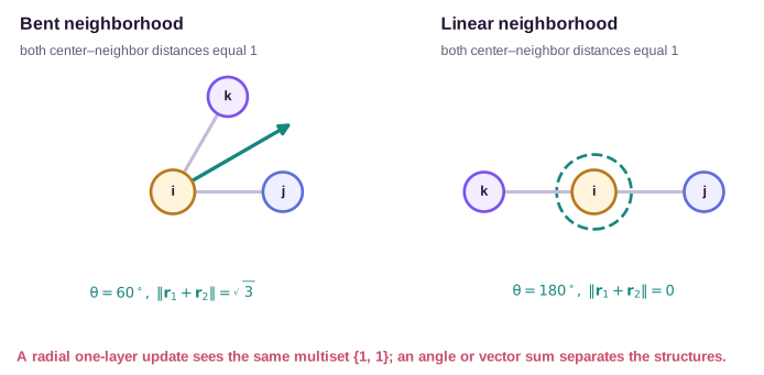
\[\mathbf{x}_1=(1,0), \qquad \mathbf{x}_2=(\cos\theta,\sin\theta).\]We will compare a bent geometry with \(\theta=60^\circ\) against a linear geometry with \(\theta=180^\circ\). Both give the center the same multiset of radial inputs, \(\{\!\{1,1\}\!\}\). Their neighbor–neighbor distances, angles, coordinate displacements, and vector sums differ. SchNet-like radial filtering, DimeNet/GemNet-style angle processing, EGNN coordinate updates, and PaiNN-like scalar/vector messages will all see the same two configurations with declared toy parameters.
Geometry fixes the transformation law
Let atom \(i\) have position \(\mathbf{x}_i\in\mathbb{R}^3\) and invariant attributes \(\mathbf{h}_i\), such as element type. A Euclidean transformation acts as
\[\mathbf{x}_i' = \mathbf{Q}\mathbf{x}_i + \mathbf{b},\]where \(\mathbf{Q}^{\mathsf T}\mathbf{Q}=\mathbf{I}\) and \(\mathbf{b}\in\mathbb{R}^3\). Orthogonal matrices with determinant \(+1\) are rotations; determinant \(-1\) includes reflections.
The target chooses the output law. An energy is invariant,
\[E(\{\mathbf{Q}\mathbf{x}_i+\mathbf{b}\})=E(\{\mathbf{x}_i\}),\]while a polar vector such as force is equivariant,
\[\mathbf{F}_i(\{\mathbf{Q}\mathbf{x}_j+\mathbf{b}\}) =\mathbf{Q}\mathbf{F}_i(\{\mathbf{x}_j\}).\]The post Symmetry and Equivariance for Geometric Data derives these transformation laws, composition closure, parity, and safe nonlinearities. Here we use those results to compare concrete geometric layers.
Relative displacement removes translation:
\[\mathbf{r}_{ij}=\mathbf{x}_j-\mathbf{x}_i, \qquad \mathbf{r}_{ij}'=\mathbf{Q}\mathbf{r}_{ij}.\]Its length \(r_{ij}=\lVert\mathbf{r}_{ij}\rVert\) is invariant because
\[(r_{ij}')^2 =\mathbf{r}_{ij}^{\mathsf T}\mathbf{Q}^{\mathsf T}\mathbf{Q}\mathbf{r}_{ij} =r_{ij}^2.\]All architectures below combine these two primitives: invariant functions choose coefficients, and relative vectors supply directions. The difference is where each architecture converts vectors to scalars and whether a direction survives the conversion.
Scalarization turns geometry into numbers
Scalarization maps coordinates to quantities unchanged by the chosen group. Distances use two atoms. Bond angles use three. Torsions use four. Each step exposes a higher-order relation while discarding the global pose.
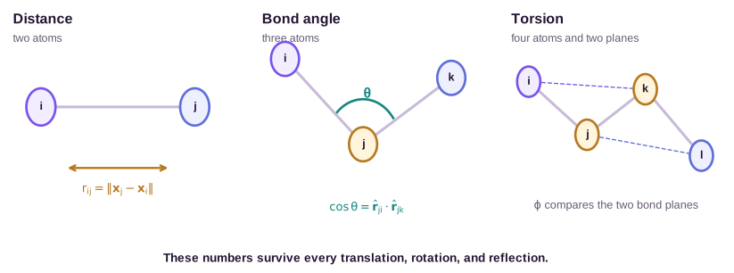
For neighbors \(j\) and \(k\) of center \(i\), their bond angle satisfies
\[\cos\theta_{jik} =\hat{\mathbf{r}}_{ij}^{\mathsf T}\hat{\mathbf{r}}_{ik}, \qquad \hat{\mathbf{r}}_{ij}=\frac{\mathbf{r}_{ij}}{r_{ij}}.\]Both directions rotate by \(\mathbf{Q}\), so their inner product remains fixed. A torsion compares the normals of two bond planes. Its sign changes under reflection unless the convention discards orientation, which is why chirality requires more than ordinary \(O(3)\)-invariant distances and unsigned angles.
Complete distances reconstruct centered coordinates
The information content of distances can be stated exactly. Suppose \(n\) labeled points form the rows of \(\mathbf{X}\in\mathbb{R}^{n\times3}\). Let \(\boldsymbol{\Delta}\) contain squared pair distances,
\[\Delta_{ij}=\lVert\mathbf{x}_i-\mathbf{x}_j\rVert^2,\]and let
\[\mathbf{J}=\mathbf{I}-\frac{1}{n}\mathbf{1}\mathbf{1}^{\mathsf T}\]be the centering matrix. Translating the point cloud so that its centroid is zero gives \(\mathbf{J}\mathbf{X}=\mathbf{X}\). Its Gram matrix is \(\mathbf{B}=\mathbf{X}\mathbf{X}^{\mathsf T}\), with entries \(B_{ij}=\mathbf{x}_i^{\mathsf T}\mathbf{x}_j\).
Expand one squared distance:
\[\Delta_{ij}=B_{ii}+B_{jj}-2B_{ij}.\]In matrix form,
\[\boldsymbol{\Delta} =\operatorname{diag}(\mathbf{B})\mathbf{1}^{\mathsf T} +\mathbf{1}\operatorname{diag}(\mathbf{B})^{\mathsf T} -2\mathbf{B}.\]Multiplying by \(\mathbf{J}\) on both sides removes the first two terms because \(\mathbf{J}\mathbf{1}=\mathbf{0}\). Centering also gives \(\mathbf{J}\mathbf{B}\mathbf{J}=\mathbf{B}\). Therefore
\[\boxed{\mathbf{B}=-\frac{1}{2}\mathbf{J}\boldsymbol{\Delta}\mathbf{J}}.\]This double-centering identity underlies classical multidimensional scaling (Torgerson, 1952). If \(\boldsymbol{\Delta}\) is an exact Euclidean distance matrix for points in three dimensions, \(\mathbf{B}\) is positive semidefinite with rank at most three. Write its positive eigendecomposition as
\[\mathbf{B}=\mathbf{U}_3\boldsymbol{\Lambda}_3\mathbf{U}_3^{\mathsf T}.\]One centered reconstruction is
\[\widehat{\mathbf{X}} =\mathbf{U}_3\boldsymbol{\Lambda}_3^{1/2}.\]Any \(\widehat{\mathbf{X}}\mathbf{Q}\) with \(\mathbf{Q}\in O(3)\) has the same Gram matrix and distances. Translation was removed by centering, and the remaining ambiguity is an orthogonal transformation: rotation or reflection. Distances therefore cannot choose handedness. No coordinate reconstruction can recover which member of an enantiomeric pair was supplied when the complete distance matrices agree.
The controlled geometries make the reconstruction concrete. For the bent case, all three pair distances equal one, so
\[\boldsymbol{\Delta}_{\mathrm{bent}} =\begin{bmatrix}0&1&1\\1&0&1\\1&1&0\end{bmatrix}.\]Double-centering gives a rank-two Gram matrix with positive eigenvalues \(1/2\) and \(1/2\): an equilateral triangle in a centered frame. For the linear case,
\[\boldsymbol{\Delta}_{\mathrm{linear}} =\begin{bmatrix}0&1&1\\1&0&4\\1&4&0\end{bmatrix},\]and the centered Gram matrix has one positive eigenvalue \(2\). The complete distance matrix separates the shapes by both the missing distance \(r_{12}\) and reconstruction rank.
The matrices make the rank statement directly checkable. For the bent triangle,
\[\mathbf{B}_{\mathrm{bent}} =\begin{bmatrix} 1/3&-1/6&-1/6\\ -1/6&1/3&-1/6\\ -1/6&-1/6&1/3 \end{bmatrix}.\]Every row sums to zero because the reconstructed coordinates are centered. The all-ones vector has eigenvalue zero, while any two independent vectors orthogonal to it have eigenvalue \(1/2\). For the linear configuration, the original coordinates already have zero centroid, so
\[\mathbf{B}_{\mathrm{linear}} =\begin{bmatrix} 0&0&0\\ 0&1&-1\\ 0&-1&1 \end{bmatrix}.\]Only direction \((0,1,-1)\) has nonzero eigenvalue, namely \(2\). Taking square roots of these eigenvalues reconstructs a two-dimensional triangle or a one-dimensional line without choosing an absolute pose.
Exact Euclidean consistency is part of the reconstruction claim. Experimental or predicted distances may violate triangle inequalities or make \(\mathbf{B}\) have negative eigenvalues. Keeping the largest positive eigenvalues then gives a classical-scaling approximation, not an exact reconstruction. A model that predicts all pair distances still needs compatibility constraints if those distances are supposed to describe one realizable geometry.
Completeness is global; a layer is local
The center does not receive either complete matrix in a one-layer radial GNN. It receives only the distances on incident edges. In both controlled configurations,
\[\left\{\!\left\{r_{01},r_{02}\right\}\!\right\} =\{\!\{1,1\}\!\}.\]Every permutation-invariant function of that multiset returns the same center update. The missing distance follows from the law of cosines,
\[r_{12}^2=1^2+1^2-2\cos\theta.\]It equals \(1\) at \(60^\circ\) and \(4\) at \(180^\circ\). If edge \((1,2)\) exists, its distance can first update nodes 1 and 2 and reach the center on a later layer. If that edge is absent from the sparse interaction graph, depth alone never creates its distance. An explicit angle, a complete radius graph, a coordinate operation, or a vector channel changes what is locally accessible.
The update schedule also matters. In a synchronous message-passing layer, node 0 receives the previous states of nodes 1 and 2. Even if those neighbors are connected, their states have not yet incorporated \(r_{12}\) during the same layer. The earliest route through edge \((1,2)\) takes two layers: one to encode that edge at a neighbor and one to transmit the result to the center. A directed-edge architecture can make the two incident edges interact in one block because its basic state and neighborhood are different.
A two-layer radial route to the missing distance
A fixed scalar calculation shows the depth requirement without appealing to a receptive-field slogan. Include all three undirected edges, initialize \(h_0^{(0)}=h_1^{(0)}=h_2^{(0)}=1\), and use the deliberately simple radial update
\[h_i^{(t+1)} =\sum_{j\in\mathcal{N}(i)}r_{ij}h_j^{(t)}.\]This is a valid invariant radial layer with filter \(W(r)=r\) and no residual term. At the center, the first-layer output is identical:
\[h_0^{(1)}=r_{01}+r_{02}=2.\]The neighbors already differ. In the bent triangle, \(r_{12}=1\), so
\[h_1^{(1)}=r_{10}+r_{12}=2, \qquad h_2^{(1)}=2.\]In the linear geometry, \(r_{12}=2\), so both neighbor states equal 3. The center can use that difference only on the second layer:
\[h_{0,\mathrm{bent}}^{(2)} =1\cdot2+1\cdot2=4, \qquad h_{0,\mathrm{linear}}^{(2)} =1\cdot3+1\cdot3=6.\]The complete distances distinguished the configurations immediately; this node-centered radial architecture needed two synchronous layers to route the decisive entry to node 0. If edge \((1,2)\) is removed and only the star remains, every edge distance, feature, and adjacency relation supplied to the radial network is identical across the two inputs. Then no depth or parameter choice can separate them. The coordinate arrays differ, but that architecture never reads the missing part of the arrays.
Complete distances use \(O(n^2)\) storage, and dense eigendecomposition for reconstruction costs \(O(n^3)\). A sparse graph with \(m\) directed edges stores \(O(m)\) distances. The savings come from not exposing every global relation. Scalarization can be complete as a representation while a particular scalar network remains incomplete as a local computation.
Distance-conditioned message passing
SchNet uses continuous radial filters to turn each edge distance into a channel-wise message weight (Schütt et al., 2017). A simplified layer is
\[\mathbf{h}_i^{+} =\mathbf{h}_i +\sum_{j\in\mathcal{N}(i)} \mathbf{h}_j\odot\mathbf{W}(r_{ij}).\]Element embeddings and hidden features are invariant. Since \(\mathbf{W}\) depends only on distance, the output is invariant as well.
Radial bases turn one distance into a smooth coordinate
A filter network rarely consumes a raw distance alone. One common expansion uses Gaussian radial basis functions
\[e_k(r)=\exp\!\left[-\beta(r-\mu_k)^2\right], \qquad k=1,\ldots,B.\]The centers \(\mu_k\) tile the interaction range, while \(\beta\) controls overlap. With \(\beta=4\) and centers \((0.5,1.0,1.5)\), a unit edge becomes
\[\mathbf{e}(1) =\left(e^{-1},1,e^{-1}\right) \approx(0.368,1,0.368).\]The expansion does not add geometric information: it is still a deterministic function of \(r\). It gives the learned filter several smooth local coordinates in which narrow and broad radial responses are easier to approximate. Very narrow bases resolve fine radial changes but leave gaps between centers. Very broad bases overlap smoothly but blur short length scales. Learned layers after the expansion decide which resolution matters.
Finite-range models also multiply messages by a cutoff envelope. A cosine cutoff is
\[c(r)= \begin{cases} \frac{1}{2}\left[\cos\!\left(\frac{\pi r}{r_c}\right)+1\right], & r<r_c,\\ 0, & r\geq r_c. \end{cases}\]Both \(c(r_c)\) and the left derivative \(c'(r_c)\) are zero. If the remaining filter is bounded and differentiable, energy and its first coordinate derivative approach zero continuously as an edge leaves the neighborhood. A hard cutoff can jump the energy or force when an atom crosses \(r_c\). The envelope improves boundary smoothness; it does not represent interactions beyond the cutoff.
Smoothness order determines which physical derivatives behave well. The cosine envelope is continuously differentiable at the cutoff after extension by zero, but its second derivative generally jumps there. That is enough to prevent a force discontinuity when the network predicts energy, but not enough to guarantee a continuous Hessian. Vibrational frequencies and force-constant calculations may require a higher-order polynomial envelope whose additional derivatives vanish at \(r_c\). Cutoff design is therefore part of the differentiability of the learned potential, not only a neighbor-list optimization.
The radial output on the controlled neighborhood
Set one scalar channel with \(h_0=0\), \(h_1=h_2=1\), and declare the learned filter value \(W(1)=2\). The center update is
\[h_0^{+}=1\cdot2+1\cdot2=4\]for both the bent and linear geometries. This equality holds for every radial filter, not only our chosen value, because both incident distances and neighbor features match. Optimization cannot infer \(\theta\) from an input that is identical at this layer.
The cost makes radial processing attractive. With \(m\) directed edges and \(B\) radial basis functions, evaluating the basis costs \(O(mB)\). Channel mixing depends on implementation, but a dense \(C_s\)-channel edge transform typically adds a term on the order of \(O(mC_s^2)\), often reduced by factorization. Geometry enters once per edge rather than once per neighbor pair.
Invariant pair energy gives central conservative forces
An invariant scalar model can still produce vector forces. Start with the transparent pair energy
\[E(\mathbf{X})=\sum_{i<j}u(r_{ij}).\]Since
\[\nabla_{\mathbf{x}_i}r_{ij} =\frac{\mathbf{x}_i-\mathbf{x}_j}{r_{ij}} =-\hat{\mathbf{r}}_{ij},\]the force on atom \(i\) is
\[\mathbf{F}_i =-\nabla_{\mathbf{x}_i}E =\sum_{j\neq i}u'(r_{ij})\hat{\mathbf{r}}_{ij}.\]Every pair contribution lies along the line joining the atoms. The corresponding contribution on \(j\) is opposite, so \(\mathbf{F}_{ij}=-\mathbf{F}_{ji}\) and \(\sum_i\mathbf{F}_i=\mathbf{0}\). Pairwise centrality also makes the pair torque vanish. Translation and rotation invariance imply the same total-force and total-torque identities for general differentiable many-body energies, as derived in the symmetry post.
The signs follow from differentiating the same pair term with respect to its two endpoints. With \(\hat{\mathbf r}_{ij}=(\mathbf x_j-\mathbf x_i)/r_{ij}\),
\[\mathbf F_{i\leftarrow j}=u'(r_{ij})\hat{\mathbf r}_{ij}, \qquad \mathbf F_{j\leftarrow i}=-u'(r_{ij})\hat{\mathbf r}_{ij}.\]Their sum is zero before any graph-level aggregation. Their torque about an arbitrary origin is also zero:
\[\begin{aligned} \boldsymbol\tau_{ij} &=\mathbf x_i\times\mathbf F_{i\leftarrow j} +\mathbf x_j\times\mathbf F_{j\leftarrow i}\\ &=(\mathbf x_i-\mathbf x_j) \times\left[u'(r_{ij})\hat{\mathbf r}_{ij}\right] =\mathbf{0}, \end{aligned}\]because \(\mathbf x_i-\mathbf x_j\) is parallel to \(\hat{\mathbf r}_{ij}\). These cancellations justify zero total internal force and torque for the pair model; equivariance by itself would not.
Take the star energy \(E=\frac12r_{01}^2+\frac12r_{02}^2\). Then \(u'(1)=1\) and
\[\mathbf{F}_0 =\hat{\mathbf{r}}_{01}+\hat{\mathbf{r}}_{02}.\]The bent center force is \((3/2,\sqrt{3}/2)\) with magnitude \(\sqrt{3}\); the linear center force is zero. The energy has the same value, \(1\), in both configurations, but its coordinate gradient differs because the edge directions differ. Invariance of a scalar output does not mean its derivatives lack direction.
The remaining atom forces make the cancellation explicit. In the bent geometry,
\[\mathbf F_1=(-1,0), \qquad \mathbf F_2=\left(-\frac12,-\frac{\sqrt{3}}{2}\right),\]and these sum with \(\mathbf F_0\) to zero. In the linear geometry, \(\mathbf F_1=(-1,0)\) and \(\mathbf F_2=(1,0)\) while \(\mathbf F_0=\mathbf{0}\). Bending changes how the two central forces interfere, but it does not change action–reaction on either edge.
For time-independent Newtonian dynamics \(m_i\ddot{\mathbf{x}}_i=\mathbf{F}_i\), exact gradient forces conserve total mechanical energy in continuous time:
\[\frac{d}{dt}\left( \sum_i\frac12m_i\lVert\dot{\mathbf{x}}_i\rVert^2+E \right) =\sum_i\dot{\mathbf{x}}_i^{\mathsf T} \left(m_i\ddot{\mathbf{x}}_i+\nabla_{\mathbf{x}_i}E\right) =0.\]A finite-step integrator introduces numerical error, and a time-dependent external field can inject energy. “Conservative by construction” refers to the learned force field \(-\nabla E\), not to exact conservation under every simulation protocol.
Direction can remain scalar
Angle-aware networks expose three-body geometry while keeping hidden channels invariant. DimeNet stores scalar states on directed edges and lets an edge update depend on a neighboring directed edge and the angle between them (Gasteiger et al., 2020). A schematic update is
\[\mathbf{m}_{ji}^{+} =U\!\left( \mathbf{m}_{ji}, \sum_{k\in\mathcal{N}(j)\setminus\{i\}} M(\mathbf{m}_{kj},r_{ji},r_{kj},\theta_{kji}) \right).\]Distances and angles are invariant, so arbitrary scalar networks can process them. GemNet extends the directional construction to richer edge interactions and establishes universality under its stated geometric setting (Klicpera et al., 2021).
The angle-aware output on the same neighborhood
Use the scalar statistic
\[a_0=\sum_{1\leq j<k\leq2} \hat{\mathbf{r}}_{0j}^{\mathsf T}\hat{\mathbf{r}}_{0k} =\cos\theta\]as a one-channel toy angle message with unit learned coefficient. It gives
\[a_0^{\mathrm{bent}}=\frac12, \qquad a_0^{\mathrm{linear}}=-1.\]The radial calculation returned 4 for both inputs; this angle channel separates them before any additional propagation. A real DimeNet layer expands radial and angular functions and mixes directed-edge states, but the source of the distinction is the same inner product.
One cosine is complete for a single unsigned angle in \([0,\pi]\) because cosine is one-to-one on that interval. A sum of cosines is not complete for a many-neighbor environment. Angle pairs with cosines \(\{\!\{1/2,-1/2\}\!\}\) and \(\{\!\{1/4,-1/4\}\!\}\) both sum to zero. Directed-edge states, multiple angular basis functions, and nonlinear interactions retain more than this toy sum. The calculation isolates the first directional statistic; it is not a claim that one scalar describes an arbitrary neighborhood.
Angle access increases enumeration. If node \(i\) has degree \(d_i\), the number of ordered neighbor pairs centered at \(i\) is \(d_i(d_i-1)\). Across the graph,
\[T=\sum_i d_i(d_i-1).\]For roughly regular degree \(k\), radial edges scale as \(m\approx nk\) while triplets scale as \(T\approx nk(k-1)\). Angular basis evaluation with \(B_a\) features costs \(O(TB_a)\) before channel mixing. The quadratic dependence on local degree can dominate around dense atoms even when the graph is globally sparse. Directional scalar networks spend that cost to make a relation between two incident edges available in one block.
Vector channels keep orientation alive
A scalar/vector network stores invariant channels \(\mathbf{s}_i\in\mathbb{R}^{C_s}\) and vector channels \(\mathbf{V}_i\in\mathbb{R}^{3\times C_v}\). Under \(\mathbf{Q}\in O(3)\),
\[\mathbf{s}_i'=\mathbf{s}_i, \qquad \mathbf{V}_i'=\mathbf{Q}\mathbf{V}_i.\]Vector addition, invariant scalar multiplication, norms, and inner products preserve these laws. Componentwise nonlinearities on Cartesian components generally do not. Rather than repeat the counterexample and closure proof, the safe and unsafe nonlinearities subsection of the symmetry chapter gives the exact calculation.
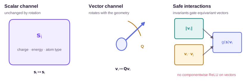
The useful loop is scalar to vector to scalar. An invariant coefficient \(w_{ij}\) lifts an edge direction into a vector message,
\[\mathbf{v}_i=\sum_j w_{ij}\hat{\mathbf{r}}_{ij}.\]Its squared norm creates an invariant containing cross-edge angles:
\[\begin{aligned} \lVert\mathbf{v}_i\rVert^2 &=\sum_j w_{ij}^2 +2\sum_{j<k}w_{ij}w_{ik} \hat{\mathbf{r}}_{ij}^{\mathsf T}\hat{\mathbf{r}}_{ik}. \end{aligned}\]The cross terms are exactly weighted cosines. A vector channel can therefore accumulate directions cheaply along edges, then expose angular correlations through a norm or inner product. It does not need to enumerate every triplet explicitly for this particular statistic, although it compresses the collection into only the vector moments that its channels retain.
With \(w_{01}=w_{02}=1\), the controlled vector is
\[\mathbf{v}_0^{\mathrm{bent}} =\left(\frac32,\frac{\sqrt{3}}{2}\right), \qquad \mathbf{v}_0^{\mathrm{linear}}=\mathbf{0}.\]Scalarizing gives \(\lVert\mathbf{v}_0\rVert^2=3\) versus \(0\). A scalar gate such as \(g(q)=1/(1+q)\) then returns the equivariant vector \(g(q)\mathbf{v}_0\). In the bent case it is \((3/8,\sqrt{3}/8)\); in the linear case it remains zero. The scalar affects magnitude, while the vector supplies orientation.
Vector storage is \(3nC_v\) numbers instead of \(nC_v\) scalar numbers. Forming direction-weighted messages costs \(O(3mC_v)\) after invariant coefficients are available. Learned channel mixing can add \(O(mC_v^2)\) or lower factorized costs depending on the architecture. Vector channels avoid explicit triplet enumeration for some correlations, but they do not encode every pair of directions unless enough channels and interactions preserve the required moments.
A first vector moment has exact collisions. Three unit directions separated by 120 degrees sum to zero, as do two opposite unit directions. Their neighbor counts and angle multisets differ, but the single vector \(\sum_j\hat{\mathbf r}_{ij}\) is identical. Scalar count channels already separate this two-versus-three example. Richer vector channels can weight directions by neighbor features or radial responses, while higher-order tensor features retain angular moments that a polar vector cannot. Avoiding explicit triplets exchanges enumeration for a compressed directional summary, not for a complete local geometry.
EGNN derives vectors from coordinate differences
The E(n)-Equivariant Graph Neural Network (EGNN) retains invariant node features and uses coordinates themselves as the equivariant state (Satorras et al., 2021). It computes an invariant edge message
\[\mathbf{m}_{ij} =\phi_e(\mathbf{h}_i,\mathbf{h}_j, \lVert\mathbf{x}_i-\mathbf{x}_j\rVert^2,\mathbf{a}_{ij})\]and an invariant scalar coefficient \(\alpha_{ij}=C\phi_x(\mathbf{m}_{ij})\). Coordinates update as
\[\mathbf{x}_i^{+} =\mathbf{x}_i +\sum_{j\neq i}(\mathbf{x}_i-\mathbf{x}_j)\alpha_{ij}.\]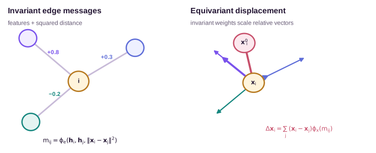
The transformation proof
Transform inputs by \(\widetilde{\mathbf{x}}_i=\mathbf{Q}\mathbf{x}_i+\mathbf{b}\). Squared distances and invariant features do not change, so \(\widetilde\alpha_{ij}=\alpha_{ij}\). Relative coordinates satisfy
\[\widetilde{\mathbf{x}}_i-\widetilde{\mathbf{x}}_j =\mathbf{Q}(\mathbf{x}_i-\mathbf{x}_j).\]The transformed update is therefore
\[\begin{aligned} \widetilde{\mathbf{x}}_i^{+} &=\mathbf{Q}\mathbf{x}_i+\mathbf{b} +\sum_j\mathbf{Q}(\mathbf{x}_i-\mathbf{x}_j)\alpha_{ij}\\ &=\mathbf{Q}\mathbf{x}_i^{+}+\mathbf{b}. \end{aligned}\]The proof holds for every learned parameter value because the architecture restricts learned outputs to invariant coefficients.
The coordinate output on the controlled neighborhood
Set \(\alpha_{01}=\alpha_{02}=1/2\) and inspect the center displacement,
\[\Delta\mathbf{x}_0 =\frac12(\mathbf{x}_0-\mathbf{x}_1) +\frac12(\mathbf{x}_0-\mathbf{x}_2).\]The bent and linear outputs are
\[\Delta\mathbf{x}_0^{\mathrm{bent}} =\left(-\frac34,-\frac{\sqrt{3}}{4}\right), \qquad \Delta\mathbf{x}_0^{\mathrm{linear}}=\mathbf{0}.\]Their magnitudes are \(\sqrt{3}/2\) and zero. A 90-degree rotation sends the bent displacement to \((\sqrt{3}/4,-3/4)\) without changing either coefficient. Radial scalar filtering could not distinguish the center states in one layer; EGNN keeps the same radial coefficient but multiplies it by the two actual directions.
Equivariance does not guarantee centroid or energy conservation
The unweighted centroid changes by
\[\overline{\mathbf{x}}^{+}-\overline{\mathbf{x}} =\frac{1}{n}\sum_i\sum_{j\neq i} (\mathbf{x}_i-\mathbf{x}_j)\alpha_{ij}.\]Group the two directed terms for each unordered pair. Their contribution is
\[(\mathbf{x}_i-\mathbf{x}_j)(\alpha_{ij}-\alpha_{ji}).\]Thus symmetric coefficients \(\alpha_{ij}=\alpha_{ji}\) preserve the centroid. Standard equivariance alone does not require this symmetry because messages may depend asymmetrically on receiver and sender features. For masses \(m_i\), preservation of the center of mass requires the stronger pair condition \(m_i\alpha_{ij}=m_j\alpha_{ji}\).
Calling a coordinate displacement a “force” does not create momentum conservation. If the update represents an internal force or velocity increment, antisymmetric pair contributions are needed for zero total momentum change. If it merely refines latent coordinates in a generative model, centroid preservation may be a convenient gauge choice rather than a physical law.
An EGNN coordinate field can also be equivariant without being conservative. Conservativity requires a scalar energy \(E\) with \(\Delta\mathbf{x}_i\propto-\nabla_{\mathbf{x}_i}E\), or equivalent integrability conditions on the full Jacobian of the field. The transformation proof above supplies neither. A separately parameterized equivariant vector field can have nonzero circulation. Equivariance controls how the field transforms; an energy gradient controls whether work is path independent.
Two particles give a minimal counterexample. Let
\[\Delta\mathbf{x}_1=\mathbf{x}_1-\mathbf{x}_2, \qquad \Delta\mathbf{x}_2=\mathbf{0}.\]The update is translation equivariant and \(O(3)\) equivariant: a rigid motion rotates the first displacement and leaves the second at zero. Its centroid changes because the directed coefficients are not symmetric. It cannot be the gradient of any twice-differentiable scalar potential, since the cross-Jacobian blocks disagree:
\[\frac{\partial\Delta\mathbf{x}_1}{\partial\mathbf{x}_2} =-\mathbf{I}, \qquad \frac{\partial\Delta\mathbf{x}_2}{\partial\mathbf{x}_1} =\mathbf{0}.\]A Hessian must be symmetric under exchange of these blocks. This field satisfies the geometric transformation law while failing both pair action–reaction and integrability.
Coordinate aggregation adds only \(O(3m)\) arithmetic and \(O(3n)\) coordinate state after edge coefficients are computed. The invariant message network still carries its scalar-channel cost. EGNN obtains a useful equivariant state without storing many vector channels, but coordinates represent one geometric vector per node rather than an arbitrary bank of directional memories.
PaiNN stores vectors as hidden features
PaiNN keeps coordinates fixed and stores dedicated scalar and vector features at every atom (Schütt et al., 2021). A simplified message separates the two paths:
\[\begin{aligned} \mathbf{m}_i^s &=\sum_{j\in\mathcal{N}(i)} \phi_s(\mathbf{s}_j,r_{ij}),\\ \mathbf{M}_i^v &=\sum_{j\in\mathcal{N}(i)} \left[ \mathbf{V}_j\mathbf{W}_{vv}(\mathbf{s}_j,r_{ij}) +\hat{\mathbf{r}}_{ij}\mathbf{w}_{vs}(\mathbf{s}_j,r_{ij})^{\mathsf T} \right]. \end{aligned}\]The learned coefficients depend on invariant inputs. Existing vector features and unit edge directions rotate by \(\mathbf{Q}\), so the message rotates by \(\mathbf{Q}\). Norms and inner products then pass invariant summaries back to scalar channels, whose nonlinear updates can gate the next vector state.
Scalar-to-vector-to-scalar coupling on the controlled geometry
Initialize one vector channel to zero and set the declared scalar-to-vector coefficient on both unit edges to one. PaiNN’s directional term gives exactly
\[\mathbf{M}_0^v =\hat{\mathbf{r}}_{01}+\hat{\mathbf{r}}_{02}.\]The bent message is \((3/2,\sqrt{3}/2)\) and the linear message is zero. Now choose the toy scalar update
\[s_0^{+}=s_0+\lVert\mathbf{M}_0^v\rVert^2.\]With \(s_0=0\), the scalar outputs are 3 and 0. The network has converted two scalar radial coefficients into a vector, allowed the directions to interfere, and returned the interference to a nonlinear scalar path. DimeNet exposed the same distinction through an explicitly enumerated cosine; PaiNN formed a vector moment and obtained the cosine cross term when taking its norm.
A direct vector readout can map \(\mathbf{M}_0^v\) to a force, dipole, or displacement while preserving equivariance. Such a head is not automatically conservative. PaiNN can instead predict an invariant energy from scalar channels and differentiate it, recovering the gradient guarantee described earlier. Output type and conservation are separate decisions even inside one architecture.
The controlled vector gives a concrete failure. If a direct head reports \(\widehat{\mathbf F}_0=\mathbf M_0^v\) and sets the two neighbor forces to zero, every output rotates correctly. In the bent geometry, however, the predicted total force is \((3/2,\sqrt{3}/2)\) rather than zero. Equivariance has been satisfied, while internal momentum balance has not. An energy-gradient head or an explicitly antisymmetric edge-force construction adds the missing constraint.
Four representative design points
The controlled calculation holds the geometry and toy coefficients fixed enough to expose where direction enters:
| design | center input used in one update | declared toy output: bent / linear | first missing or retained relation |
|---|---|---|---|
| SchNet-like radial | \(r_{01}=r_{02}=1\), \(W(1)=2\) | scalar \(4\) / \(4\) | loses the angle at this layer |
| DimeNet/GemNet-like scalar | \(\cos\theta\) with unit coefficient | scalar \(1/2\) / \(-1\) | exposes the edge-pair angle |
| EGNN coordinate | relative vectors with \(\alpha=1/2\) | displacement \((-3/4,-\sqrt{3}/4)\) / \(\mathbf{0}\) | retains direction in coordinates |
| PaiNN-like scalar/vector | unit direction messages | vector \((3/2,\sqrt{3}/2)\) / \(\mathbf{0}\); scalar \(3\) / \(0\) | retains a directional moment and scalarizes it later |
The numerical values are not predictions of the named trained models. They follow from stated toy parameters. The architectural facts are which inputs each update accepts, which transformation types its hidden states carry, and which correlations become available without another propagation step.
Cost follows the same boundary. Let \(m\) be the number of directed edges, \(d_i\) the node degrees, \(C_s\) scalar width, and \(C_v\) vector width.
| operation | geometric enumeration | leading geometric state/work |
|---|---|---|
| radial edge filtering | \(m\) edges | \(O(mB)\) for \(B\) radial bases; \(O(nC_s)\) scalar state |
| angle-aware scalar filtering | \(\sum_i d_i(d_i-1)\) ordered triplets | angular-basis work proportional to triplets; directed-edge scalar state |
| EGNN coordinate update | \(m\) relative vectors | \(O(3m)\) coordinate aggregation; \(O(3n)\) coordinate state |
| scalar/vector messaging | \(m\) relative directions | \(O(3mC_v)\) direction weighting; \(O(3nC_v)\) vector state, plus channel mixing |
The table omits model-specific dense transforms, attention, and batching constants. It isolates the geometric multiplier. Angle-aware models pay in neighbor pairs. Coordinate models store one position vector. Vector-channel models pay three Cartesian components for every vector channel.
For scale, take \(n=1000\) atoms with directed degree \(k=32\). Radial processing visits about \(m=nk=32{,}000\) directed edges. Ordered angle processing visits
\[T=nk(k-1)=992{,}000\]triplets, about 31 times as many geometric interactions before basis width and channel transforms. With \(C_v=32\), vector state stores \(3nC_v=96{,}000\) floating-point values, compared with \(32{,}000\) values for 32 scalar channels. These numbers do not predict wall-clock time, but they show which multiplier grows when coordination number or vector width increases.
What directional information buys
Directional information buys a shorter computational path, not a magical new geometry. The complete Euclidean distance matrix already determines our three-point shape up to \(O(3)\). But the sparse radial center update sees only two unit distances and collides. An explicit angle, an equivariant coordinate sum, or a vector moment separates the bent and linear neighborhoods in one update.
The final design choice should separate four questions that are often mixed together.
| representation choice | complete in principle? | local accessibility | natural output | conservation guarantee |
|---|---|---|---|---|
| complete labeled distance matrix | determines centered coordinates up to \(O(3)\) when Euclidean | global \(O(n^2)\) input; reconstruction is dense | invariant scalars after ordinary processing | none unless output is an energy and forces are differentiated |
| sparse radial scalar network | generally incomplete because only selected edge distances enter | one edge per layer; omitted distances never appear without changing the graph | invariant node or graph scalars | gradient forces are conservative; direct scalar output alone says nothing about dynamics |
| angle-aware scalar network | locally includes selected three-body invariants, not every global geometry | triplets available in one block; long-range relations still need depth | invariant energies and other scalars | conservative only when forces are derived from the invariant energy |
| EGNN coordinate update | coordinates themselves retain the represented point configuration | relative directions available on each chosen edge | equivariant coordinates or vectors plus invariant features | equivariance alone gives neither centroid preservation nor a conservative field |
| scalar/vector network | retained vector moments preserve selected directional information | directions persist across layers in \(C_v\) channels | invariant scalars and direct equivariant vectors | direct vector heads need not be conservative; energy-gradient heads are |
Representation completeness concerns what could be reconstructed from all encoded variables. Local accessibility concerns which of those variables meet inside a layer. Output type concerns whether the final quantity is invariant or equivariant. Conservation concerns whether a vector field comes from a time-independent invariant energy and whether its pair or global symmetries enforce zero total force and torque. No single “equivariant” label answers all four.
A radial energy model is a good choice when pair distances and depth expose the needed chemistry and conservative forces matter. Angle-aware scalar processing is attractive when local bond geometry is decisive and triplet cost is acceptable. EGNN is economical when coordinates are latent states to refine or transport. Scalar/vector channels fit tasks where direction must survive several interactions or feed a vector output directly. Higher-order spherical features extend the same logic beyond ordinary vectors; Spherical Equivariant Layers for 3D Atomic Systems develops that machinery.
Scalar and vector networks solve the same geometric problem at different points in the computation. The useful question is not whether direction exists somewhere in the input. It is whether the architecture makes the required directional correlation accessible, stable, and compatible with the output and physical constraints of the task.
References
- Torgerson, W. S. (1952). Multidimensional Scaling: I. Theory and Method. Psychometrika, 17, 401–419. DOI. ↩
- Schütt, K. T., Kindermans, P.-J., Sauceda, H. E., Chmiela, S., Tkatchenko, A., & Müller, K.-R. (2017). SchNet: A Continuous-filter Convolutional Neural Network for Modeling Quantum Interactions. NeurIPS 2017. Proceedings. ↩
- Gasteiger, J., Groß, J., & Günnemann, S. (2020). Directional Message Passing for Molecular Graphs. ICLR 2020. OpenReview. ↩
- Klicpera, J., Becker, F., & Günnemann, S. (2021). GemNet: Universal Directional Graph Neural Networks for Molecules. NeurIPS 2021. OpenReview. ↩
- Satorras, V. G., Hoogeboom, E., & Welling, M. (2021). E(n) Equivariant Graph Neural Networks. ICML 2021. PMLR. ↩
- Schütt, K. T., Unke, O. T., & Gastegger, M. (2021). Equivariant Message Passing for the Prediction of Tensorial Properties and Molecular Spectra. ICML 2021. PMLR. ↩