Steerable Features and Tensor Products

Adapted from my 2025 Machine Learning for Molecules and Geometric Deep Learning lectures. This article stays concrete—low-order Cartesian algebra and one complete typed message layer—while Symmetry and Equivariance motivates the transformation laws and Spherical Equivariant Layers develops the Wigner-basis implementation.

An equivariant network cannot treat every hidden array as an ordinary feature vector. Some channels are scalars and should stay fixed under rotation. Others encode directions and should rotate as vectors. Higher-order channels contain angular patterns whose components mix in less familiar but equally precise ways.

This creates a type system for geometry. Every feature carries a rule for how it transforms, and every layer must preserve those rules. Linear maps alone can mix channels of the same type, but they cannot create the interactions that make a deep network expressive. The missing operation is multiplication.

The Clebsch–Gordan tensor product is multiplication for rotation-typed features. It couples two input types, decomposes their pairwise products into valid output types, and exposes exactly which couplings are allowed. Combined with spherical harmonics on edges and invariant gates, it gives a reusable recipe for building nonlinear equivariant layers.

Rotation equivariance imposes a feature type system

Let \(\mathbf{f}^{(\ell)}\) denote a feature of type \(\ell\). Under a three-dimensional rotation \(\mathbf{R}\in SO(3)\), it transforms as

\[\mathbf{f}^{(\ell)} \mapsto \mathbf{D}^{(\ell)}(\mathbf{R}) \mathbf{f}^{(\ell)}.\]

The matrix \(\mathbf{D}^{(\ell)}(\mathbf{R})\) is the degree-\(\ell\) irreducible representation of \(SO(3)\). It has size \((2\ell+1)\times(2\ell+1)\). “Irreducible” means that no fixed change of basis can split these components into smaller subspaces that remain independent under every rotation.

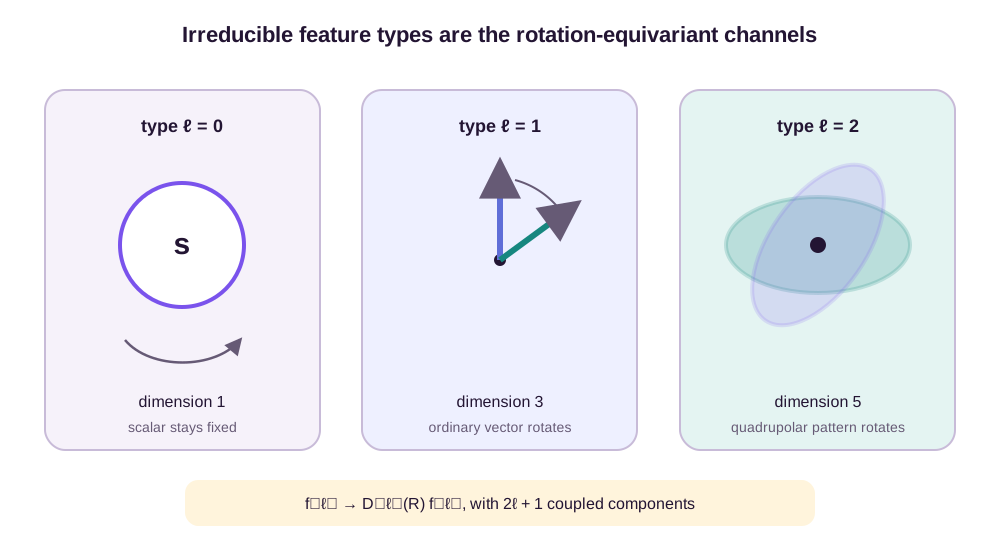
The first three types have concrete interpretations:

• Type \(\ell=0\) has one component. Its representation is the number one, so it is a scalar.
• Type \(\ell=1\) has three components. It transforms as an ordinary vector.
• Type \(\ell=2\) has five components. It describes a quadrupolar angular pattern, equivalent to the independent components of a symmetric traceless \(3\times3\) tensor.

The feature ladder below emphasizes that each type is one coupled geometric block rather than a bag of scalar coordinates.

A network usually stores multiple channels of each type. If there are \(C_\ell\) type-\(\ell\) channels, the feature block has shape

\[\mathbf{F}^{(\ell)} \in \mathbb{R}^{C_\ell\times(2\ell+1)}.\]

The channel index selects different learned features. The magnetic index \(m\in\{-\ell,\ldots,\ell\}\) selects components within one geometric feature. Rotations mix the \(m\) components but do not mix learned channels. Confusing these two axes is a common source of broken implementations.

Why linear weights live on the channel axis

The restriction on a typed linear layer follows from the representation, rather than from an implementation convention. Write the full type-\(\ell\) space as

\[\mathbb{R}^{C_\ell}\otimes V_\ell,\]

where \(V_\ell\) is the \((2\ell+1)\)-dimensional irreducible carrier space. Rotation acts as

\[\rho_\ell(\mathbf R) = \mathbf I_{C_\ell}\otimes\mathbf D^{(\ell)}(\mathbf R).\]

A linear map \(\mathbf T\) from \(C_\ell\) input copies to \(C_\ell'\) output copies is equivariant only if it commutes with every rotation:

\[\mathbf T (\mathbf I_{C_\ell}\otimes\mathbf D^{(\ell)}(\mathbf R)) = (\mathbf I_{C_\ell'}\otimes\mathbf D^{(\ell)}(\mathbf R)) \mathbf T \qquad\text{for every }\mathbf R\in SO(3).\]

View \(\mathbf T\) as a \(C_\ell'\times C_\ell\) block matrix, with each block mapping \(V_\ell\) to itself. Every block must commute with every \(\mathbf D^{(\ell)}(\mathbf R)\). For the real integer-degree irreducible representations of \(SO(3)\) used here, Schur’s-lemma intuition says such a block is a scalar multiple of the identity. Thus

\[\boxed{\mathbf T=\mathbf W^{(\ell)}\otimes\mathbf I_{2\ell+1}}.\]

The learned matrix \(\mathbf W^{(\ell)}\) may mix multiplicity channels arbitrarily, but one coefficient acts identically on all magnetic components. The scope matters. This conclusion assumes a linear intertwiner between copies of one irreducible real \(SO(3)\) type. Additional parity labels under \(O(3)\) split the blocks further, and nonlinear tensor products are not constrained to this form.

Maps between inequivalent types vanish under the same assumptions. A linear map from one scalar to one vector that commuted with every rotation would have to choose a vector fixed by every rotation; only the zero vector qualifies. Biases obey the same rule: an unconstrained bias is legal for type 0, while a nonzero fixed vector bias would select a preferred direction.

Cohen and Welling (2017) describe this representation-theoretic organization as a type system for steerable networks (Cohen & Welling, 2017). The type system turns “do not break rotation symmetry” into a concrete restriction on each weight block.

Spherical harmonics turn directions into typed features

The direction from node \(i\) to node \(j\) is

\[\widehat{\mathbf{r}}_{ij} = \frac{\mathbf{r}_j-\mathbf{r}_i} {\lVert\mathbf{r}_j-\mathbf{r}_i\rVert}.\]

Its Cartesian coordinates form a type-1 vector, but one direction can generate every angular type. The degree-\(\ell\) spherical harmonics collect \(2\ell+1\) functions into a vector

\[\mathbf{Y}^{(\ell)} \left( \widehat{\mathbf{r}} \right) = \left[ Y_{\ell,-\ell}(\widehat{\mathbf{r}}), \ldots, Y_{\ell,\ell}(\widehat{\mathbf{r}}) \right]^{\mathsf{T}}.\]

Under rotation, this vector transforms through the same irreducible representation:

\[\mathbf{Y}^{(\ell)} \left( \mathbf{R}\widehat{\mathbf{r}} \right) = \mathbf{D}^{(\ell)}(\mathbf{R}) \mathbf{Y}^{(\ell)} \left( \widehat{\mathbf{r}} \right),\]

up to the chosen real or complex harmonic convention. Spherical harmonics therefore convert edge direction into a feature with a declared rotation type.

Distance supplies the complementary invariant information. A learnable radial function \(R_c^{(\ell)}(r_{ij})\) depends only on

\[r_{ij}=\lVert\mathbf{r}_j-\mathbf{r}_i\rVert.\]

Multiplying the angular feature by this scalar produces a steerable filter:

\[\mathbf{F}_{c}^{(\ell)} \left( \mathbf{r}_{ij} \right) = R_c^{(\ell)}(r_{ij}) \mathbf{Y}^{(\ell)} \left( \widehat{\mathbf{r}}_{ij} \right).\]

The filter separates what changes under rotation from what does not. The spherical harmonic carries orientation, while the radial network learns how interaction strength varies with distance. Tensor Field Networks use exactly this construction to obtain rotation-, translation-, and permutation-equivariant point-cloud layers (Thomas et al., 2018).

Low degrees without basis conventions

The spherical anchor develops normalized harmonic bases. For the low-order algebra here, Cartesian equivalents make the typing visible without committing to a phase or normalization convention. For a unit direction \(\mathbf n=(n_x,n_y,n_z)\), use

\[\mathcal Y^{(0)}(\mathbf n)=1, \qquad \mathcal Y^{(1)}(\mathbf n)=\mathbf n, \qquad \mathcal Y^{(2)}(\mathbf n)= \mathbf n\mathbf n^{\mathsf T}-\frac{1}{3}\mathbf I.\]

The last object is symmetric and traceless, so it has five independent components. It is a Cartesian realization of type 2. These expressions omit conventional normalization constants, which change lengths but not transformation types.

Evaluate them on the coordinate directions. For \(\mathbf e_x=(1,0,0)\),

\[\mathcal Y^{(1)}(\mathbf e_x)= \begin{bmatrix}1\\0\\0\end{bmatrix}, \qquad \mathcal Y^{(2)}(\mathbf e_x)= \begin{bmatrix} 2/3&0&0\\ 0&-1/3&0\\ 0&0&-1/3 \end{bmatrix}.\]

For \(\mathbf e_y=(0,1,0)\), the positive \(2/3\) entry moves from the first diagonal position to the second. Let \(\mathbf R_z\) be a 90-degree rotation about the \(z\) axis. Since \(\mathbf R_z\mathbf e_x=\mathbf e_y\),

\[\mathcal Y^{(1)}(\mathbf e_y) =\mathbf R_z\mathcal Y^{(1)}(\mathbf e_x),\]

and

\[\mathcal Y^{(2)}(\mathbf e_y) = \mathbf R_z \mathcal Y^{(2)}(\mathbf e_x) \mathbf R_z^{\mathsf T}.\]

The type-1 components rotate once; the type-2 tensor rotates on both indices. For the diagonal direction \(\mathbf n=(\mathbf e_x+\mathbf e_y)/\sqrt2\),

\[\mathcal Y^{(2)}(\mathbf n)= \begin{bmatrix} 1/6&1/2&0\\ 1/2&1/6&0\\ 0&0&-1/3 \end{bmatrix}.\]

The off-diagonal entries record orientation that no single scalar distance contains. Under inversion, \(\mathcal Y^{(1)}(-\mathbf n)=-\mathcal Y^{(1)}(\mathbf n)\) while \(\mathcal Y^{(2)}(-\mathbf n)=\mathcal Y^{(2)}(\mathbf n)\). This is the low-degree parity rule \((-1)^\ell\) in Cartesian form.

Linear maps cannot create new geometric interactions

Typed linear maps are necessary but not sufficient. A stack of linear equivariant maps remains linear, and mixing only channels of the same type cannot create a scalar from two vectors or a higher-order angular feature from lower-order inputs.

An ordinary componentwise nonlinearity is not a solution. For a type-1 vector, ReLU generally fails the equivariance equation:

\[\operatorname{ReLU} \left( \mathbf{R}\mathbf{v} \right) \neq \mathbf{R} \operatorname{ReLU} \left( \mathbf{v} \right).\]

A two-dimensional subcase shows the failure. Let

\[\mathbf{v} = \begin{bmatrix} 1\\-1 \end{bmatrix}, \qquad \mathbf{R} = \begin{bmatrix} 0&-1\\ 1&0 \end{bmatrix}.\]

Then \(\operatorname{ReLU}(\mathbf{R}\mathbf{v})=(1,1)^{\mathsf{T}}\), while \(\mathbf{R}\operatorname{ReLU}(\mathbf{v})=(0,1)^{\mathsf{T}}\). ReLU treats coordinate axes as physically meaningful, so it destroys the vector transformation law.

We need a nonlinear operation that knows the types of both inputs and outputs. Products provide that operation because rotations distribute over multiplication. The remaining problem is to reorganize those products into irreducible blocks.

The tensor product is equivariant but reducible

Consider a type-\(\ell_1\) feature \(\mathbf{x}^{(\ell_1)}\) and a type-\(\ell_2\) feature \(\mathbf{y}^{(\ell_2)}\). Their ordinary tensor product contains every pairwise component product:

\[\mathbf{x}^{(\ell_1)} \otimes \mathbf{y}^{(\ell_2)}.\]

After rotation,

\[\left( \mathbf{D}^{(\ell_1)}(\mathbf{R})\mathbf{x}^{(\ell_1)} \right) \otimes \left( \mathbf{D}^{(\ell_2)}(\mathbf{R})\mathbf{y}^{(\ell_2)} \right) = \left( \mathbf{D}^{(\ell_1)}(\mathbf{R}) \otimes \mathbf{D}^{(\ell_2)}(\mathbf{R}) \right) \left( \mathbf{x}^{(\ell_1)} \otimes \mathbf{y}^{(\ell_2)} \right).\]

The product is already equivariant. Its problem is organization: the Kronecker-product representation is reducible. Its components contain several irreducible types mixed together.

Clebsch–Gordan coefficients define the change of basis that separates those types. The type-\(\ell\) output is

\[z_m^{(\ell)} = \sum_{m_1=-\ell_1}^{\ell_1} \sum_{m_2=-\ell_2}^{\ell_2} C^{\ell m}_{\ell_1 m_1,\ell_2 m_2} x_{m_1}^{(\ell_1)} y_{m_2}^{(\ell_2)}.\]

Here, \(C^{\ell m}_{\ell_1 m_1,\ell_2 m_2}\) is a fixed Clebsch–Gordan coefficient. It is not learned. The learned parameters decide which channels interact and how strongly; the coefficients decide how component products must combine to transform as type \(\ell\).

The change of basis preserves dimension. Before decomposition, the tensor product has

\[(2\ell_1+1)(2\ell_2+1)\]

components. The proposed irreducible blocks contain

\[\sum_{\ell=\lvert\ell_1-\ell_2\rvert}^{\ell_1+\ell_2}(2\ell+1) =(2\ell_1+1)(2\ell_2+1).\]

To verify the sum, assume \(\ell_1\geq\ell_2\). There are \(2\ell_2+1\) terms, and their average degree is \(\ell_1\). Summing \(2\ell+1\) therefore gives \((2\ell_2+1)(2\ell_1+1)\). No component is created or discarded by the Clebsch–Gordan transform; it only reorganizes the product space.

Equivariance of each projected block follows from the intertwining identity for the fixed projection \(\mathbf C_\ell\):

\[\mathbf C_\ell \left( \mathbf D^{(\ell_1)}(\mathbf R) \otimes \mathbf D^{(\ell_2)}(\mathbf R) \right) = \mathbf D^{(\ell)}(\mathbf R)\mathbf C_\ell.\]

Applying the product representation and then projecting gives the same result as projecting first and rotating the declared output type. This fixed algebra is the closure step that lets tensor products sit safely inside a network.

Selection rules remove impossible couplings

Most coefficients in the component formula are zero. Two rules state which outputs can survive.

The triangle rule restricts the output degree:

\[\lvert\ell_1-\ell_2\rvert \leq \ell \leq \ell_1+\ell_2.\]

The magnetic-index rule requires

\[m=m_1+m_2.\]

The magnetic-index rule is written in the conventional complex spherical basis. A real spherical-harmonic basis is obtained by mixing the \(m\) and \(-m\) components, so its coefficient table has a different sparsity pattern. The basis-independent statement is the triangle rule and the existence of the intertwining projection above.

The allowed output representation is therefore

\[\mathbf{D}^{(\ell_1)} \otimes \mathbf{D}^{(\ell_2)} \cong \bigoplus_{\ell=\lvert\ell_1-\ell_2\rvert}^{\ell_1+\ell_2} \mathbf{D}^{(\ell)}.\]

The coupling diagram below collects the degree, magnetic-index, and parity checks in one place.

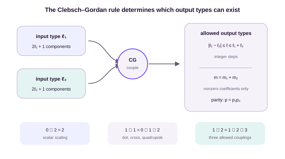
These rules are the geometric analogue of shape checking. A scalar times a type-2 feature can only produce type 2:

\[0\otimes2=2.\]

A vector times a type-2 feature can produce three types:

\[1\otimes2 = 1\oplus2\oplus3.\]

No parameter choice can make a type-0 output from this pair because type 0 is absent from the decomposition.

Reflections add one more label. An \(O(3)\) feature carries parity \(p\in\{+1,-1\}\), which says whether it stays fixed or changes sign under inversion. Tensor products multiply parity:

\[p_{\text{out}} = p_1p_2.\]

The degree-\(\ell\) spherical harmonic has parity \((-1)^\ell\). A polar vector is odd, while the cross product of two polar vectors is an even axial vector. Two features can share the same rotation degree and still differ under reflection, so parity must be tracked when the task has full \(O(3)\) symmetry.

Parity and degree impose separate checks. Coupling a polar vector \((\ell=1,p=-1)\) with an odd type-1 edge harmonic gives output parity \(+1\). The allowed rotational degrees are still \(0,1,2\), but their parity-even outputs are a scalar, an axial vector, and an even rank-two tensor. A polar-vector output \((1,-1)\) is forbidden on this path even though degree 1 satisfies the triangle rule. It would require an additional odd factor or a different input parity.

Two vectors contain scalar, vector, and quadrupole information

The coupling

\[1\otimes1 = 0\oplus1\oplus2\]

is the most useful low-order example. Two three-dimensional vectors have a \(3\times3=9\) dimensional outer product. The Clebsch–Gordan change of basis separates it into blocks of dimensions

\[9=1+3+5.\]

In Cartesian notation, the three blocks are familiar.

The type-0 block is the trace, proportional to the dot product:

\[s=\mathbf{x}\cdot\mathbf{y}.\]

The type-1 block is the antisymmetric part, represented by the cross product:

\[\mathbf{a} = \mathbf{x}\times\mathbf{y}.\]

The type-2 block is the symmetric traceless part:

\[\mathbf{Q} = \frac{1}{2} \left( \mathbf{x}\mathbf{y}^{\mathsf{T}} +\mathbf{y}\mathbf{x}^{\mathsf{T}} \right) - \frac{1}{3} \left( \mathbf{x}\cdot\mathbf{y} \right)\mathbf{I}.\]

A complete numerical decomposition

Take

\[\mathbf x=(1,2,0)^{\mathsf T}, \qquad \mathbf y=(0,1,1)^{\mathsf T}.\]

Their outer product is

\[\mathbf M=\mathbf x\mathbf y^{\mathsf T} = \begin{bmatrix} 0&1&1\\ 0&2&2\\ 0&0&0 \end{bmatrix}.\]

The scalar and axial-vector blocks are

\[s=\mathbf x\cdot\mathbf y=2, \qquad \mathbf a=\mathbf x\times\mathbf y=(2,-1,1)^{\mathsf T}.\]

The symmetric traceless block is

\[\mathbf Q= \begin{bmatrix} -2/3&1/2&1/2\\ 1/2&4/3&1\\ 1/2&1&-2/3 \end{bmatrix}.\]

It is visibly symmetric and its diagonal sums to zero, leaving five degrees of freedom. Together, \(s\), \(\mathbf a\), and \(\mathbf Q\) contain \(1+3+5=9\) numbers subject to the block constraints, exactly matching the nine entries of \(\mathbf M\).

The decomposition is invertible. Define the skew matrix \([\mathbf a]_\times\) by \([\mathbf a]_\times\mathbf z=\mathbf a\times\mathbf z\). The vector triple-product identity gives

\[[\mathbf x\times\mathbf y]_\times = \mathbf y\mathbf x^{\mathsf T} - \mathbf x\mathbf y^{\mathsf T}.\]

The symmetric part of \(\mathbf M\) is \(\mathbf Q+(s/3)\mathbf I\), while its antisymmetric part is \(-[\mathbf a]_\times/2\). Therefore

\[\boxed{ \mathbf x\mathbf y^{\mathsf T} = \mathbf Q+\frac{s}{3}\mathbf I -\frac{1}{2}[\mathbf a]_\times }.\]

For our values,

\[[\mathbf a]_\times= \begin{bmatrix} 0&-1&-1\\ 1&0&-2\\ 1&2&0 \end{bmatrix},\]

and substitution reconstructs the matrix \(\mathbf M\) entry by entry. Dropping any block loses a specific part of the outer product: the trace, orientation of the antisymmetric plane, or symmetric anisotropy.

Rotation and inversion checks

Rotate both inputs by 90 degrees about the \(z\) axis. With

\[\mathbf R_z= \begin{bmatrix} 0&-1&0\\ 1&0&0\\ 0&0&1 \end{bmatrix},\]

the vectors become \(\mathbf x'=(-2,1,0)^{\mathsf T}\) and \(\mathbf y'=(-1,0,1)^{\mathsf T}\). Direct calculation gives

\[s'=2=s, \qquad \mathbf a'=(1,2,1)^{\mathsf T}=\mathbf R_z\mathbf a,\]

and

\[\mathbf Q'=\mathbf R_z\mathbf Q\mathbf R_z^{\mathsf T}.\]

The three blocks obey their declared scalar, vector, and rank-two laws. Their reconstruction gives

\[\mathbf x'\mathbf y'^{\mathsf T} = \mathbf R_z\mathbf M\mathbf R_z^{\mathsf T},\]

as it must.

Under inversion, both polar inputs change sign. Their dot product, outer product, and symmetric-traceless block remain fixed. Their cross product also remains fixed because it is axial:

\[(-\mathbf x)\times(-\mathbf y)=\mathbf x\times\mathbf y.\]

This case prevents a common type error. The degree-1 cross-product block transforms like an ordinary vector under \(SO(3)\), but it has even parity under \(O(3)\). Angular degree alone cannot encode that distinction.

The decomposition figure below shows how the three blocks partition all nine components.

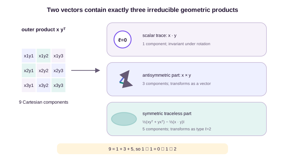
This example explains why tensor products add expressivity. A scalar-only network can measure the angle between two directions through the dot product, but it discards their oriented plane. The type-1 output keeps that orientation through the cross product. The type-2 output retains a quadrupolar pattern that neither a scalar nor a single vector can represent.

Kondor et al. (2018) make this bilinear coupling the source of nonlinearity in Clebsch–Gordan networks (Kondor et al., 2018). Repeated products can build higher-order interactions while every intermediate block retains an exact transformation type.

Equivariant nonlinearities act through invariants

Tensor products are not the only legal nonlinear operation. A scalar feature is invariant, so any ordinary activation can act on type 0:

\[s\mapsto\sigma(s).\]

A higher-order feature can be scaled by an invariant gate:

\[\mathbf{f}^{(\ell)} \mapsto \sigma(g) \mathbf{f}^{(\ell)}, \qquad g\text{ is type }0.\]

The scalar gate changes magnitude without changing the rotation law. Its value may come from a separate scalar channel, a norm, or a tensor product projected to type 0.

A norm nonlinearity makes the same idea explicit:

\[\mathbf{f}^{(\ell)} \mapsto \eta\!\left( \left\lVert \mathbf{f}^{(\ell)} \right\rVert \right) \frac{ \mathbf{f}^{(\ell)} }{ \left\lVert \mathbf{f}^{(\ell)} \right\rVert+\varepsilon }.\]

The norm is invariant, while the normalized direction remains type \(\ell\). Gated and norm-based nonlinearities are standard components of three-dimensional steerable CNNs (Weiler et al., 2018).

The \(\varepsilon\) in the denominator is more than numerical decoration. Without it, the direction is undefined at the zero feature. A gate \(\sigma(g)\mathbf f^{(\ell)}\) stays well-defined there and can change sign if the scalar gate permits signed values. A norm-rescaling map usually preserves the ray of a nonzero feature and changes only its magnitude. Neither operation creates a new angular type; a tensor product is still needed to turn, for example, two vectors into a scalar and a type-2 feature.

A componentwise activation fails because it depends on the chosen coordinate basis. A norm-dependent scalar coefficient succeeds because

\[\lVert\mathbf D^{(\ell)}(\mathbf R)\mathbf f^{(\ell)}\rVert_2 = \lVert\mathbf f^{(\ell)}\rVert_2\]

for an orthogonal real irrep basis. The safe operation is therefore a scalar function of an invariant multiplied by the whole irrep block. This is the only nonlinear principle needed here; the preceding symmetry chapter gives the broader closure argument and force/readout consequences.

Each option makes a different tradeoff. Scalar-only activations are cheap but leave higher types linear between coupling operations. Gates are efficient but cannot create a new type. Tensor products create new angular content, but their cost grows with the number of input channels and allowed coupling paths. Practical layers combine all three.

One layer couples node features with edge geometry

The pieces now assemble into a steerable message-passing layer.

For each edge \((i,j)\), compute the invariant distance \(r_{ij}\) and direction \(\widehat{\mathbf{r}}_{ij}\). A radial network and spherical harmonics produce a filter of type \(\ell_f\):

\[\mathbf{F}_{ij}^{(\ell_f)} = R^{(\ell_f)}(r_{ij}) \mathbf{Y}^{(\ell_f)} \left( \widehat{\mathbf{r}}_{ij} \right).\]

Couple a neighbor feature of type \(\ell_{\text{in}}\) with this filter and retain an allowed output type:

\[\mathbf{m}_{ij}^{(\ell_{\text{out}})} = \sum_{\ell_{\text{in}},\ell_f} w_{\ell_{\text{in}},\ell_f,\ell_{\text{out}}} (r_{ij}) \left[ \mathbf{h}_j^{(\ell_{\text{in}})} \otimes_{\mathrm{CG}} \mathbf{Y}^{(\ell_f)} \left( \widehat{\mathbf{r}}_{ij} \right) \right]^{(\ell_{\text{out}})}.\]

The bracket selects the type-\(\ell_{\text{out}}\) Clebsch–Gordan block. The learned radial weight \(w\) mixes channels and controls distance dependence. The selection rule requires

\[\lvert \ell_{\text{in}}-\ell_f \rvert \leq \ell_{\text{out}} \leq \ell_{\text{in}}+\ell_f.\]

The low-order cases give this equation a physical interpretation. Suppose node \(j\) carries a scalar charge-like feature \(q_j\) and the edge filter has type \(\ell_f=1\). The only allowed output is type 1:

\[0\otimes1=1.\]

Up to basis normalization, the message is

\[\mathbf{m}_{ij}^{(1)} \propto R(r_{ij})q_j \widehat{\mathbf{r}}_{ij}.\]

The scalar controls magnitude and the edge direction controls orientation. Rotating the molecule rotates the message.

Now suppose node \(j\) carries a vector \(\mathbf{v}_j\). Coupling it to the same type-1 edge filter gives

\[1\otimes1=0\oplus1\oplus2.\]

The scalar output is proportional to the radial projection

\[\mathbf{v}_j\cdot\widehat{\mathbf{r}}_{ij}.\]

The vector output is proportional to the oriented tangential component

\[\mathbf{v}_j\times\widehat{\mathbf{r}}_{ij},\]

and the type-2 output is their symmetric traceless product. One neighbor feature and one edge direction therefore yield three geometrically distinct messages. Learned channel weights can retain all three, suppress some paths, or send them to different downstream channels without changing their transformation laws.

A complete two-neighbor typed update

Fix one center with two unit-distance neighbors. Let their edge directions be

\[\mathbf n_1=\mathbf e_x, \qquad \mathbf n_2=\mathbf e_y.\]

Neighbor 1 carries invariant scalar \(q_1=2\) and polar vector \(\mathbf v_1=(1,1,0)^{\mathsf T}\). Neighbor 2 carries \(q_2=-1\) and \(\mathbf v_2=(2,0,0)^{\mathsf T}\). Set every radial coefficient to one. These declared values isolate the typed algebra from the radial network.

Use four allowed paths:

\[\begin{aligned} m_j^{(0,+)}&=\mathbf v_j\cdot\mathbf n_j,\\ \mathbf m_j^{(1,-)}&=q_j\mathbf n_j,\\ \mathbf m_j^{(1,+)}&=\mathbf v_j\times\mathbf n_j,\\ \mathbf M_j^{(2,+)}&= \frac{\mathbf v_j\mathbf n_j^{\mathsf T} +\mathbf n_j\mathbf v_j^{\mathsf T}}{2} -\frac{\mathbf v_j\cdot\mathbf n_j}{3}\mathbf I. \end{aligned}\]

The superscripts list degree and parity. Both \(\mathbf v_j\) and \(\mathbf n_j\) are odd polar vectors. Their dot, cross, and symmetric product are even; multiplying the even scalar \(q_j\) by the odd edge direction gives an odd polar vector.

For neighbor 1, the four messages are

\[\begin{aligned} m_1^{(0,+)}&=1,\\ \mathbf m_1^{(1,-)}&=(2,0,0)^{\mathsf T},\\ \mathbf m_1^{(1,+)}&=(0,0,-1)^{\mathsf T},\\ \mathbf M_1^{(2,+)}&= \begin{bmatrix} 2/3&1/2&0\\ 1/2&-1/3&0\\ 0&0&-1/3 \end{bmatrix}. \end{aligned}\]

For neighbor 2,

\[\begin{aligned} m_2^{(0,+)}&=0,\\ \mathbf m_2^{(1,-)}&=(0,-1,0)^{\mathsf T},\\ \mathbf m_2^{(1,+)}&=(0,0,2)^{\mathsf T},\\ \mathbf M_2^{(2,+)}&= \begin{bmatrix} 0&1&0\\ 1&0&0\\ 0&0&0 \end{bmatrix}. \end{aligned}\]

Neighbor summation gives

\[\begin{aligned} m_i^{(0,+)}&=1,\\ \mathbf m_i^{(1,-)}&=(2,-1,0)^{\mathsf T},\\ \mathbf m_i^{(1,+)}&=(0,0,1)^{\mathsf T},\\ \mathbf M_i^{(2,+)}&= \begin{bmatrix} 2/3&3/2&0\\ 3/2&-1/3&0\\ 0&0&-1/3 \end{bmatrix}. \end{aligned}\]

Every sum stays within one type. The two degree-1 channels remain separate because their parities differ. An \(SO(3)\)-only layer could mix them: proper rotations do not distinguish polar from axial vectors. An \(O(3)\) layer cannot add them without breaking reflection equivariance.

Let the invariant gate be \(g=\operatorname{sigmoid}(m_i^{(0,+)})=\operatorname{sigmoid}(1)\approx0.731\). A gated polar state becomes

\[\mathbf h_{i,\mathrm{new}}^{(1,-)} =g\mathbf m_i^{(1,-)} \approx(1.462,-0.731,0)^{\mathsf T}.\]

The axial and type-2 blocks can be gated by the same scalar while keeping their own transformation laws. A scalar graph readout may sum \(m_i^{(0,+)}\) over centers. A polar-vector target such as force may read out \(\mathbf h_{i,\mathrm{new}}^{(1,-)}\). An axial target must use the \((1,+)\) channel instead.

Rotate the entire neighborhood by 90 degrees about \(z\). Dot products and the gate stay at 1 and 0.731. The polar aggregate becomes

\[\mathbf R_z(2,-1,0)^{\mathsf T}=(1,2,0)^{\mathsf T},\]

so the gated readout becomes \((0.731,1.462,0)^{\mathsf T}\). The axial aggregate \((0,0,1)\) remains fixed under this particular rotation, and the type-2 aggregate transforms by conjugation. This checks the full edge coupling, aggregation, nonlinearity, and readout on actual values.

Sum messages over neighbors:

\[\mathbf{m}_i^{(\ell)} = \sum_{j\in\mathcal{N}(i)} \mathbf{m}_{ij}^{(\ell)}.\]

Summation is permutation-invariant and preserves the rotation type because it adds features that transform through the same matrix. A type-preserving channel mix and an invariant gate then produce the next node state.

The layer diagram below places these typed operations in their message-passing order.

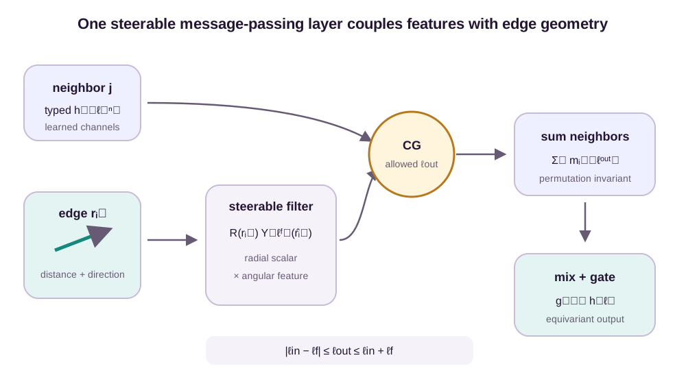
Every step has a distinct symmetry role. Relative positions remove translation. Spherical harmonics encode rotation. Clebsch–Gordan coefficients couple types. Neighbor summation removes ordering. Scalar gates add nonlinearity without choosing a coordinate axis.

For an invariant graph target such as molecular energy, the final readout uses type-0 channels. Vector or tensor targets read out the corresponding types. Intermediate higher-order channels can still improve a scalar prediction because later tensor products can couple them back to type 0.

Angular resolution and cost are coupled

The maximum degree \(L_{\max}\) limits the angular frequencies the network can represent. Increasing it adds finer directional structure, but each type has \(2\ell+1\) components and participates in more tensor-product paths. Computational cost therefore grows through both representation size and coupling count.

Count storage before counting FLOPs

For one node, the exact number of stored real feature values is

\[d_{\mathrm{node}} = \sum_{\ell=0}^{L_{\max}}C_\ell(2\ell+1).\]

If every degree has the same channel count \(C\), the sum of odd dimensions gives

\[d_{\mathrm{node}}=C(L_{\max}+1)^2.\]

With \(C=32\), scalar-only features store 32 values per node. Keeping degrees 0 and 1 stores \(32(1+3)=128\). Extending through degree 2 stores 288, and through degree 3 stores 512. These are representation values, not parameter counts. For \(N\) nodes, activation storage begins at \(N d_{\mathrm{node}}\) before edge messages, gradients, batching, and optimizer state.

Coupling count grows separately. Ignore parity and suppose input, filter, and output degrees all range from 0 through \(L_{\max}\). Count a degree triple \((\ell_{\mathrm{in}},\ell_f,\ell_{\mathrm{out}})\) whenever it satisfies the triangle rule. The numbers of allowed triples are

\(L_{\max}\)	allowed degree paths
0	1
1	5
2	15
3	34

For \(L_{\max}=1\), the five paths are \(0\otimes0\to0\), \(0\otimes1\to1\), \(1\otimes0\to1\), and the two retained parts \(1\otimes1\to0,1\). The type-2 output of \(1\otimes1\) is truncated. At \(L_{\max}=2\), ten additional degree paths become available, including the missing type-2 block and couplings involving a type-2 input or filter. Parity labels remove paths whose product parity does not match the requested output.

What a path costs

For one allowed path with \(C_{\mathrm{in}}\) input channels, \(C_f\) filter channels, and \(C_{\mathrm{out}}\) output channels, an unfactorized learned channel tensor contains on the order of

\[C_{\mathrm{in}}C_fC_{\mathrm{out}}\]

coefficients. The geometric contraction also applies fixed Clebsch–Gordan coefficients to magnetic components. A naive dense contraction can scale with the product

\[(2\ell_{\mathrm{in}}+1)(2\ell_f+1)(2\ell_{\mathrm{out}}+1),\]

but selection-rule sparsity, precomputed coefficients, path-specific channel mixing, and factorization change the constant and sometimes the effective scaling. These expressions are leading bookkeeping terms, not exact runtime claims for a library kernel. Memory movement, neighbor count, batching, and hardware utilization often dominate small low-degree products.

With uniform channel count \(C\) and every path retained, the unfactorized channel parameter term grows like the path count times \(C^3\): one block at \(L_{\max}=0\), five at 1, and fifteen at 2. Practical layers rarely allocate equal width to every degree or a full three-way channel tensor to every path. Higher degrees often receive fewer channels, and radial networks may generate path weights rather than a separate filter-channel axis.

More types are not automatically better. A model can gain capacity by adding channels at low degree, by increasing radial resolution, or by stacking more coupling layers. These choices represent different kinds of complexity. High degree adds angular detail within one layer; depth composes lower-order interactions; channel multiplicity stores more learned patterns of the same type.

Depth and degree are complementary rather than interchangeable. Two type-1 features can create type 2 in one product. If the layer truncates back to \(L_{\max}=1\), that five-dimensional block is discarded before the next layer. Deeper products can still build many-body scalar and vector functions from retained low degrees, but they cannot recover the discarded intermediate as an explicit type-2 state. Conversely, a shallow high-degree layer exposes fine angular structure but may not compose information across several graph hops.

The right truncation depends on the target, neighborhood size, and data regime. Raising \(L_{\max}\) increases angular bandwidth and cost immediately. Adding depth increases interaction order and receptive field but also adds optimization and repeated-message costs. Neither operation guarantees better accuracy. A controlled comparison should hold channel budget or runtime roughly fixed and ask which missing interaction each change makes accessible.

The useful design question is which geometric interactions the target needs. Scalar energies may benefit from vector and type-2 intermediates even though the output is invariant. A force model must retain type-1 information to the output. Reflection-sensitive targets require parity labels rather than only \(SO(3)\) degrees.

The worked layer shows what this design choice means at the level of one edge. The scalar neighbor feature set the magnitude of a polar message. The vector neighbor feature and edge direction produced an invariant projection, an axial response, and a symmetric anisotropy. Aggregation preserved each type, and one invariant gate controlled all of them without selecting an axis. Nothing in that calculation depended on an architecture name.

The type system also states what the layer deliberately cannot do. It cannot linearly turn a scalar into a direction, mix polar and axial vectors under reflections, or retain a type-2 product after truncating it away. Those exclusions are the symmetry guarantee and the approximation budget at the same time.

The resulting architecture is not a generic MLP with rotation augmentation. It is a typed program. Irreducible representations define the data types, spherical harmonics create typed edge inputs, Clebsch–Gordan products implement legal multiplication, and invariant gates provide stable nonlinear control. The companion Spherical Equivariant Layers post continues from this algebra to detailed Wigner-matrix conventions, computational strategies, and architecture families.

References

• Cohen, T. S., & Welling, M. (2017). Steerable CNNs. ICLR. ↩
• Thomas, N., Smidt, T., Kearnes, S., Yang, L., Li, L., Kohlhoff, K., & Riley, P. (2018). Tensor Field Networks: Rotation- and Translation-Equivariant Neural Networks for 3D Point Clouds. arXiv:1802.08219. ↩
• Weiler, M., Geiger, M., Welling, M., Boomsma, W., & Cohen, T. S. (2018). 3D Steerable CNNs: Learning Rotationally Equivariant Features in Volumetric Data. NeurIPS. ↩
• Kondor, R., Lin, Z., & Trivedi, S. (2018). Clebsch–Gordan Nets: A Fully Fourier Space Spherical Convolutional Neural Network. NeurIPS. ↩