On this page
Adapted from my 2025 Geometric Deep Learning lectures. After the general symmetry framework developed in Symmetry and Equivariance for Geometric Data, a practical choice remains: select one pose, construct local frames, average over finite frames, or sample a pose distribution.
An equivariant network is usually built from equivariant layers. Every intermediate feature transforms according to a prescribed representation, and each operation preserves that rule. Frames offer another route: transform the input into one or more reference poses, apply an ordinary neural network there, then transform or average the outputs.
This architecture-agnostic recipe is appealing because the backbone can be an MLP, Transformer, or pretrained model with no built-in geometric symmetry. But the apparent simplicity moves the hard problem elsewhere. A model must choose a pose continuously, or it must average over enough poses to make the choice irrelevant. Symmetric objects make a unique continuous choice impossible.
The same tension appears locally and globally. A local frame turns vectors near an edge into invariant scalar coordinates, where an ordinary nonlinear network can process them. A global frame chooses a coordinate system for an entire point cloud. Frame averaging keeps several such choices instead of trusting one. Probabilistic symmetrization replaces a finite unweighted set by a learned distribution. Each step spends more computation to reduce the instability of choosing a single pose.
One centered four-point cloud will expose that trade throughout the post. For a parameter \(-1<\varepsilon<1\), define the unordered planar cloud
\[X_\varepsilon= \left\{ (\sqrt{1+\varepsilon},0), (-\sqrt{1+\varepsilon},0), (0,\sqrt{1-\varepsilon}), (0,-\sqrt{1-\varepsilon}) \right\}.\]Positive \(\varepsilon\) stretches the horizontal arm, negative \(\varepsilon\) stretches the vertical arm, and \(X_0\) is a fourfold-symmetric cross. This family is deliberately simple: we can calculate every pose choice exactly, yet it contains the degeneracy that makes canonicalization difficult.
Symmetry identifies an orbit, not a preferred pose
Let a group \(G\) act on an input space \(\mathcal{X}\). We write \(g\cdot x\) for the transformed input. For a three-dimensional point cloud, \(G\) might be the rotation group \(SO(3)\), the orthogonal group \(O(3)\) including reflections, or the Euclidean group with translations.
The orbit of an input \(x\) is the set of all descriptions related by the group:
\[G\cdot x=\{g\cdot x:g\in G\}.\]A rotation-invariant target is constant on this orbit. A rotation-equivariant target is not constant, but its values along the orbit are determined by one value and an output representation \(\rho_Y\):
\[f(g\cdot x)=\rho_Y(g)f(x).\]The set of orbits is the quotient space \(\mathcal{X}/G\). Passing to the quotient discards pose while retaining shape. Canonicalization tries to implement this abstract quotient by selecting one concrete representative from every orbit.
For the cross, all rotated copies \(\mathbf{R}_\theta X_\varepsilon\) belong to one \(SO(2)\) orbit for each fixed \(\varepsilon\). The quotient remembers the two arm lengths, but forgets their laboratory angle. A quarter turn maps \(X_\varepsilon\) to \(X_{-\varepsilon}\), so the sign of \(\varepsilon\) merely says which laboratory axis is longer. It is not itself a quotient coordinate. A canonicalizer tries to replace the whole orbit by a convention such as “put the long arm on the horizontal axis.”
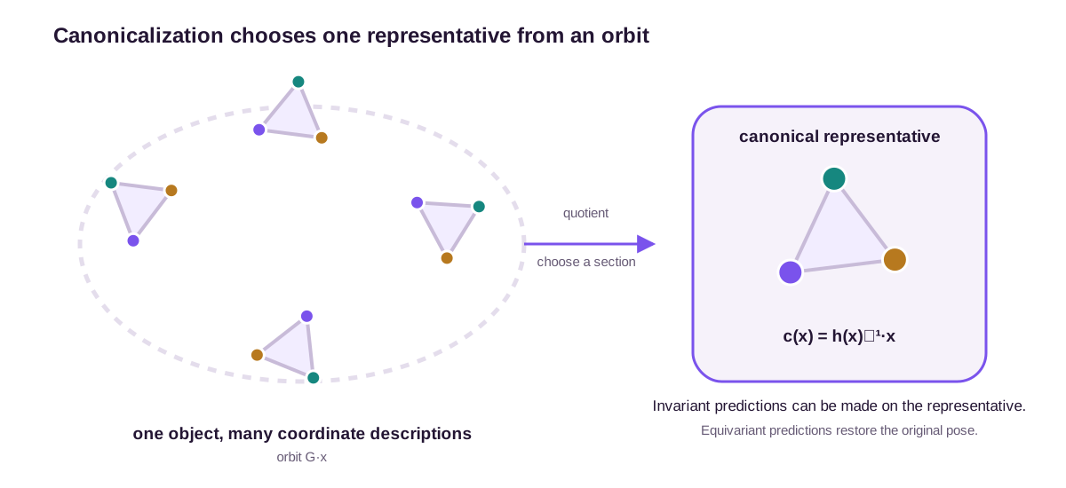
To make the construction precise, let \(h(x)\in G\) denote the pose that carries a canonical representative to \(x\). The canonicalized input is
\[c(x)=h(x)^{-1}\cdot x.\]The pose map must itself be equivariant:
\[h(g\cdot x)=g\,h(x).\]This condition makes the canonicalized input invariant:
\[c(g\cdot x) =h(g\cdot x)^{-1}\cdot(g\cdot x) =h(x)^{-1}g^{-1}g\cdot x =c(x).\]An arbitrary backbone \(\phi\) can now produce an invariant prediction
\[F_{\mathrm{inv}}(x)=\phi(c(x)).\]For an equivariant prediction, apply the output representation to restore the pose:
\[F_{\mathrm{eq}}(x) =\rho_Y(h(x))\,\phi(c(x)).\]Substituting \(h(g\cdot x)=gh(x)\) immediately gives \(F_{\mathrm{eq}}(g\cdot x)=\rho_Y(g)F_{\mathrm{eq}}(x)\). Kaba et al. use this factorization to learn the canonicalizer with a small equivariant network while leaving the main backbone unrestricted (Kaba et al., 2023).
The equation for \(h\) is stronger than choosing a repeatable preprocessing convention. It says that the pose extracted after transforming the input must be the old pose left-multiplied by the same group element. A lexicographic tie-break in laboratory coordinates can be deterministic without satisfying this law. In that case, the derivation above does not apply.
A unique canonical pose cannot always vary continuously
Canonicalization fails first at objects with nontrivial symmetry. The stabilizer of \(x\) is
\[G_x=\{g\in G:g\cdot x=x\}.\]If \(x\) is a perfectly regular tetrahedron, for example, several rotations leave it unchanged after the vertices are treated as an unordered set. Suppose a single-valued pose map \(h\) existed at such an input and satisfied the equivariance condition. For any non-identity \(s\in G_x\),
\[h(x)=h(s\cdot x)=s\,h(x).\]Left multiplication of a group element is free, so this equality would imply \(s=e\), a contradiction. A unique equivariant pose cannot be assigned to an object that does not itself have a unique pose.
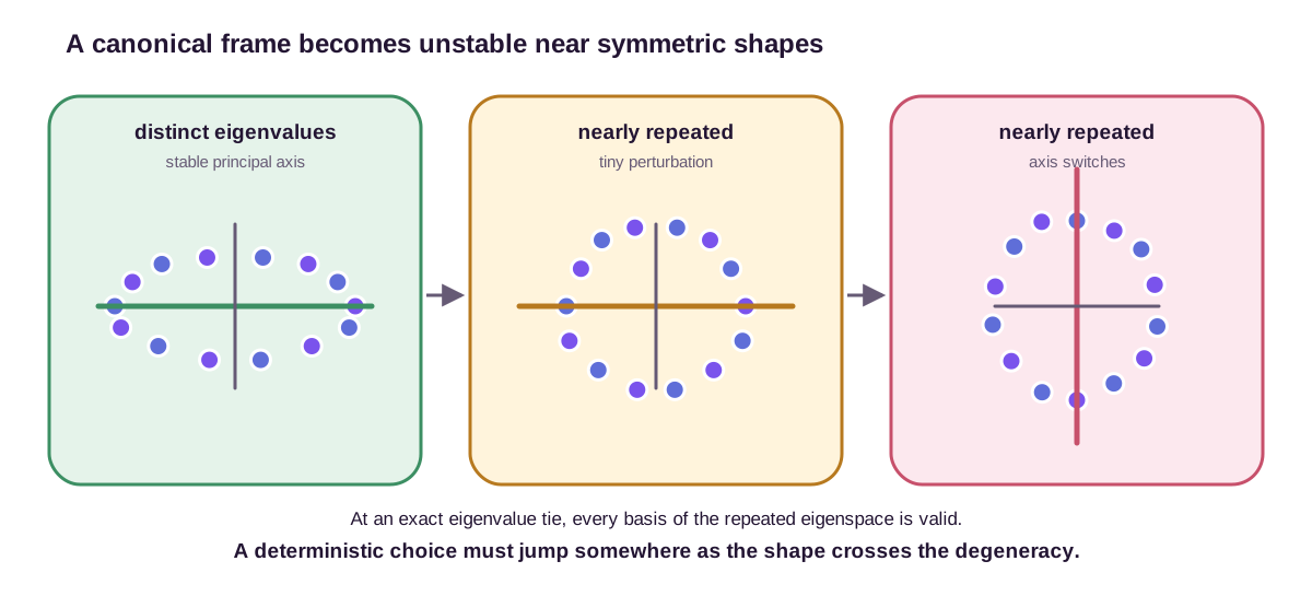
Even inputs with trivial stabilizers can approach a symmetric input. A deterministic choice must then jump somewhere. Principal-component analysis (PCA) makes the problem concrete. Center a point cloud \(\mathbf{X}\in\mathbb{R}^{N\times d}\) by subtracting its mean \(\boldsymbol{\mu}\) and form the covariance
\[\boldsymbol{\Sigma} =\frac{1}{N}\sum_{i=1}^{N} (\mathbf{x}_i-\boldsymbol{\mu}) (\mathbf{x}_i-\boldsymbol{\mu})^{\mathsf T}.\]When the eigenvalues are distinct, its eigenvectors define principal axes, though each axis still has an arbitrary sign. When two eigenvalues coincide, any orthonormal basis of their shared eigenspace is valid. Near that tie, a tiny perturbation can exchange the eigenvalue order or rotate the selected axes by a large angle.
The anisotropic cross jumps by 90 degrees
The mean of \(X_\varepsilon\) is zero, and its covariance has no off-diagonal terms because opposite points cancel. The diagonal entries are
\[\begin{aligned} \Sigma_{11} &=\frac{(1+\varepsilon)+(1+\varepsilon)}{4} =\frac{1+\varepsilon}{2},\\ \Sigma_{22} &=\frac{(1-\varepsilon)+(1-\varepsilon)}{4} =\frac{1-\varepsilon}{2}. \end{aligned}\]Therefore
\[\boldsymbol{\Sigma}_\varepsilon =\frac{1}{2} \begin{bmatrix} 1+\varepsilon&0\\ 0&1-\varepsilon \end{bmatrix}, \qquad \lambda_1-\lambda_2=\lvert\varepsilon\rvert.\]For \(\varepsilon>0\), the principal line is horizontal. For \(\varepsilon<0\), it is vertical. Take a sequence \(\varepsilon_n\downarrow0\) and another \(-\varepsilon_n\uparrow0\). The two selected principal lines approach axes separated by exactly \(\pi/2\) even though
\[\max_i\lVert\mathbf{x}_i(\varepsilon_n) -\mathbf{x}_i(-\varepsilon_n)\rVert =\left\lvert\sqrt{1+\varepsilon_n} -\sqrt{1-\varepsilon_n}\right\rvert \longrightarrow0.\]At \(\varepsilon=0\), both covariance eigenvalues equal \(1/2\), and every orthonormal basis diagonalizes the covariance. The unordered cross has a four-element rotational stabilizer, generated by a 90-degree rotation. For \(\varepsilon\ne0\) it still has a two-element stabilizer, generated by a 180-degree rotation. PCA can select its long line, but it cannot select a directed long axis equivariantly. The two signs are physically indistinguishable.
A sign convention does not remove the obstruction. Suppose an implementation asks that the first nonzero coordinate of the principal eigenvector be positive. The returned vectors are \((1,0)\) for \(\varepsilon>0\) and \((0,1)\) for \(\varepsilon<0\). They jump by 90 degrees at the tie. Rotating the same input across a coordinate boundary can also flip the sign convention without any change in shape. The rule is deterministic, yet neither continuity nor the required pose law follows from determinism.
This is not only a flaw of PCA. Dym et al. show that for common group actions there is no efficiently computable unweighted frame that preserves continuity for every function being averaged (Dym et al., 2024). The geometric obstruction is that a global continuous choice of representative—a continuous section of the quotient map—often does not exist.
Exact equivariance and numerical stability are therefore separate properties. A canonicalizer can obey the symmetry equation everywhere it is defined yet change abruptly near a degenerate configuration. A smooth backbone composed with that canonicalizer can inherit the discontinuity.
The last implication depends on the backbone. If \(\phi\) happens to give the same output for every competing canonical pose, its composition can remain continuous despite a jumping pose. For an arbitrary unrestricted \(\phi\), no such cancellation is available. The impossibility result concerns a uniformly valid wrapper, not a claim that every downstream function must jump.
Local frames avoid choosing one pose for the whole object
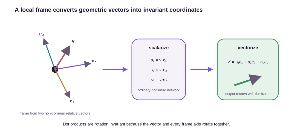
A local frame restricts the choice to a neighborhood, an edge, or a small geometric motif. This is enough to convert vector information into invariant scalars without canonicalizing the entire structure.
Consider two non-collinear relative vectors \(\mathbf{r},\mathbf{s}\in\mathbb{R}^{3}\). We can construct a right-handed orthonormal frame by Gram–Schmidt:
\[\mathbf{e}_1=\frac{\mathbf{r}}{\lVert\mathbf{r}\rVert},\] \[\widetilde{\mathbf{e}}_2 =\mathbf{s}-(\mathbf{e}_1^{\mathsf T}\mathbf{s})\mathbf{e}_1, \qquad \mathbf{e}_2 =\frac{\widetilde{\mathbf{e}}_2} {\lVert\widetilde{\mathbf{e}}_2\rVert},\] \[\mathbf{e}_3=\mathbf{e}_1\times\mathbf{e}_2.\]Collect the axes as columns of \(\mathbf{E}=[\mathbf{e}_1,\mathbf{e}_2,\mathbf{e}_3]\). Under a rotation \(\mathbf{R}\in SO(3)\), both relative vectors rotate, and the frame transforms as \(\mathbf{E}\mapsto\mathbf{R}\mathbf{E}\).
Any geometric vector \(\mathbf{v}\) can be scalarized into its coordinates in this frame:
\[\mathbf{s}_{\mathbf{v}} =\mathbf{E}^{\mathsf T}\mathbf{v} =\begin{bmatrix} \mathbf{e}_1^{\mathsf T}\mathbf{v}\\ \mathbf{e}_2^{\mathsf T}\mathbf{v}\\ \mathbf{e}_3^{\mathsf T}\mathbf{v} \end{bmatrix}.\]These coordinates are rotation invariant because
\[(\mathbf{R}\mathbf{E})^{\mathsf T}(\mathbf{R}\mathbf{v}) =\mathbf{E}^{\mathsf T}\mathbf{v}.\]An ordinary nonlinear network can process \(\mathbf{s}_{\mathbf{v}}\) along with distances, atom types, and other scalar features. If it outputs coefficients \(\mathbf{a}\), vectorization reconstructs a geometric vector:
\[\mathbf{v}'=\mathbf{E}\mathbf{a} =a_1\mathbf{e}_1+a_2\mathbf{e}_2+a_3\mathbf{e}_3.\]The reconstructed vector rotates with the input because the frame does. ClofNet uses this scalarize–process–vectorize pattern to build expressive \(SE(3)\)-equivariant graph networks from complete local frames (Du et al., 2022).
One vector triple through the complete frame
Take
\[\mathbf r=(1,0,0), \qquad \mathbf s_\theta=(\cos\theta,\sin\theta,0), \qquad \mathbf v=(1,2,3),\]with \(0<\theta<\pi\). Gram–Schmidt gives \(\mathbf e_1=(1,0,0)\), \(\widetilde{\mathbf e}_2=(0,\sin\theta,0)\), and therefore \(\mathbf E=\mathbf I\). Scalarization returns \(\mathbf E^{\mathsf T}\mathbf v=(1,2,3)\). Let the unrestricted scalar backbone return
\[\mathbf a=\phi(1,2,3) =(s_1+s_2,\,s_2s_3,\,s_1^2) =(3,6,1).\]Vectorization produces \(\mathbf v'=(3,6,1)\). Now rotate the whole triple by 90 degrees around the \(z\) axis:
\[\mathbf R= \begin{bmatrix} 0&-1&0\\ 1&0&0\\ 0&0&1 \end{bmatrix}.\]The rotated frame is \(\mathbf E'=\mathbf R\mathbf E=\mathbf R\), while the rotated vector is \(\mathbf R\mathbf v=(-2,1,3)\). Its local coordinates remain
\[(\mathbf E')^{\mathsf T}\mathbf R\mathbf v =\mathbf E^{\mathsf T}\mathbf v =(1,2,3).\]The backbone consequently returns the same coefficients \((3,6,1)\), and vectorization gives
\[\mathbf E'\mathbf a =\mathbf R(3,6,1)^{\mathsf T} =(-6,3,1)^{\mathsf T}.\]This finite calculation identifies the interface contract. The unrestricted backbone sees invariant coordinates; the geometric frame, not the backbone, carries the output transformation.
The construction has boundaries. It becomes undefined when \(\mathbf{r}=\mathbf{0}\) or when \(\mathbf{r}\) and \(\mathbf{s}\) are parallel, because the second Gram–Schmidt vector vanishes. Local-frame methods must choose geometric inputs that avoid these degeneracies, provide fallbacks, or retain several possible frames. Frames defined at neighboring nodes can also disagree; a model that mixes their coordinates needs to encode the transition from one frame to another.
The same triple quantifies the singularity. Its orthogonal residual has norm
\[\left\lVert\widetilde{\mathbf e}_2\right\rVert =\lvert\sin\theta\rvert.\]If the computed residual has perturbation \(\boldsymbol\delta\), normalization can change its direction by order
\[\frac{\lVert\boldsymbol\delta\rVert} {\lvert\sin\theta\rvert}\]for small perturbations transverse to the residual. At \(\theta=30^\circ\), the amplification denominator is \(0.5\); at \(1^\circ\), it is approximately \(0.01745\), so the same perturbation can be amplified by a factor of about \(57.3\). Approaching zero from positive angles gives \(\mathbf e_2=(0,1,0)\). Approaching from negative angles gives \(\mathbf e_2=(0,-1,0)\) and \(\mathbf e_3=(0,0,-1)\). No normalized second axis exists at \(\theta=0\) to connect the limits. A thresholded fallback only relocates the discontinuity unless the fallback is blended or averaged with a compatible transformation law.
The cross product introduces a second qualification. Under an improper rotation \(\mathbf{R}\in O(3)\) with determinant \(-1\),
\[(\mathbf{R}\mathbf{e}_1)\times(\mathbf{R}\mathbf{e}_2) =\det(\mathbf{R})\,\mathbf{R}(\mathbf{e}_1\times\mathbf{e}_2).\]The third axis is a pseudovector. A right-handed cross-product frame is naturally \(SO(3)\) equivariant, not automatically \(O(3)\) equivariant. Reflection-equivariant models must track parity or include reflected frames rather than treating every vector component as the same type.
For the vector triple, reflect across the \(xy\) plane with \(\mathbf Q=\operatorname{diag}(1,1,-1)\). The defining vectors \(\mathbf r\) and \(\mathbf s_\theta\) do not move, so rebuilding the right-handed frame returns \(\mathbf E_Q=\mathbf I\). Directly transforming the old frame would give \(\mathbf Q\mathbf E=\operatorname{diag}(1,1,-1)\). The relation is instead
\[\mathbf E_Q =\mathbf Q\mathbf E \operatorname{diag}(1,1,\det\mathbf Q),\]because the third column is axial. The reflected polar vector is \(\mathbf Q\mathbf v=(1,2,-3)\), so its third local coordinate changes from \(3\) to \(-3\). That coordinate is a pseudoscalar under reflection. Feeding all three local coordinates into an ordinary parity-blind MLP preserves \(SO(3)\) symmetry but does not, by itself, define an \(O(3)\)-equivariant map.
Group averaging symmetrizes an arbitrary function
Canonicalization evaluates the backbone once. Group averaging takes the opposite approach: evaluate it at every pose and remove the pose dependence by integration.
Assume for now that \(G\) is finite or compact, so it has a normalized invariant measure \(\mu\). For any function \(\phi:\mathcal{X}\to\mathcal{Y}\), define the equivariant symmetrization
\[(\mathcal{S}\phi)(x) =\int_G \rho_Y(g)\, \phi(g^{-1}\cdot x) \,d\mu(g).\]The invariant case uses the trivial output representation, \(\rho_Y(g)=1\). No property of \(\phi\) is required. Equivariance follows from a change of variables. For \(h\in G\), set \(g=hk\):
\[\begin{aligned} (\mathcal{S}\phi)(h\cdot x) &=\int_G \rho_Y(g)\, \phi(g^{-1}h\cdot x)\,d\mu(g)\\ &=\int_G \rho_Y(hk)\, \phi(k^{-1}\cdot x)\,d\mu(k)\\ &=\rho_Y(h)(\mathcal{S}\phi)(x). \end{aligned}\]The measure is unchanged because Haar measure is invariant under group multiplication. For a finite group, the integral is the average over all elements.
Four poses expose what averaging changes
Take the quarter-turn group \(C_4=\{e,u,u^2,u^3\}\), where \(u\) rotates by 90 degrees. To make all four stored poses distinct, imagine adding one typed marker to \(X_\varepsilon\); the marker breaks its 180-degree stabilizer without changing the covariance calculation above. Let \(x\) denote the resulting decorated cross. Evaluate one completely unrestricted scalar backbone on the four pose-normalized inputs:
| pose \(g\) | \(e\) | \(u\) | \(u^2\) | \(u^3\) |
|---|---|---|---|---|
| \(z_x(g)=\phi(g^{-1}\!\cdot x)\) | 2 | 6 | -2 | 10 |
These numbers are not assumed to obey any symmetry. They are simply a finite record of what an arbitrary backbone can return. Exact group averaging gives
\[(\mathcal S\phi)(x) =\frac{2+6-2+10}{4}=4.\]For the transformed input \(u^j\!\cdot x\), the four entries are cyclically permuted because
\[z_{u^j\cdot x}(g) =\phi(g^{-1}u^j\!\cdot x) =z_x(u^{-j}g).\]The average remains exactly \(4\) for every \(j\). The calculation does not make \(\phi\) invariant; it constructs a new invariant function by retaining the whole finite orbit and averaging its inconsistent values.
Continuous rotations make exact group averaging expensive, while the full Euclidean group is noncompact and has no normalized Haar probability measure. Geometric models usually remove translation first by centering coordinates, then average over a compact rotation or orthogonal group. Monte Carlo integration over rotations is possible, but many backbone evaluations may be needed for a low-variance result.
Exactness is always relative to the group actually integrated. Averaging these four poses enforces invariance to \(C_4\), not to every planar rotation. A full \(SO(2)\) guarantee requires the Haar integral or a special quadrature that is exact for a restricted function class. An unrestricted neural backbone has no finite angular bandlimit, so a fixed quadrature is generally an approximation to the continuous-group average.
Frame averaging replaces the group by a data-dependent set
A frame is a set-valued pose map \(\mathcal{F}:\mathcal{X}\to 2^G\) that transforms equivariantly:
\[\mathcal{F}(g\cdot x)=g\mathcal{F}(x) =\{gh:h\in\mathcal{F}(x)\}.\]Instead of averaging over all of \(G\), frame averaging uses the finite set \(\mathcal{F}(x)\):
\[(\mathcal{A}_{\mathcal{F}}\phi)(x) =\frac{1}{\lvert\mathcal{F}(x)\rvert} \sum_{h\in\mathcal{F}(x)} \rho_Y(h)\, \phi(h^{-1}\cdot x).\]The proof of equivariance is the same change-of-variables argument as for group averaging. The essential condition is not that each pose be canonical. It is that the entire set transform consistently.
PCA gives a common frame construction for a centered point cloud. If \(\mathbf{U}=[\mathbf{u}_1,\ldots,\mathbf{u}_d]\) contains principal axes with distinct eigenvalues, each eigenvector has two sign choices. Keeping all \(2^d\) signed bases produces an \(O(d)\) frame; keeping only bases with determinant \(+1\) produces the orientation-preserving subset for \(SO(d)\). Averaging removes the arbitrary sign convention. Puny et al. show that such frame averages can turn unrestricted backbones into invariant or equivariant universal approximators under their stated assumptions (Puny et al., 2022).
For the planar cross with \(\varepsilon>0\), the orientation-preserving signed PCA frame contains rotations by \(0\) and \(\pi\). For \(\varepsilon<0\), it contains rotations by \(\pi/2\) and \(3\pi/2\). These two-element sets remove the eigenvector sign. At \(\varepsilon=0\), however, the stabilizer includes every quarter turn. The frame law requires
\[\mathcal F(X_0) =u\mathcal F(X_0).\]No nonempty one- or two-element subset of \(C_4\) satisfies that equality. The smallest \(C_4\) frame at the symmetric cross is the full four-pose set. Thus the valid signed frame changes from two poses off the tie to at least four poses at the tie. Averaging resolves the sign ambiguity, but a finite unweighted construction still changes combinatorially at the eigenvalue collision.
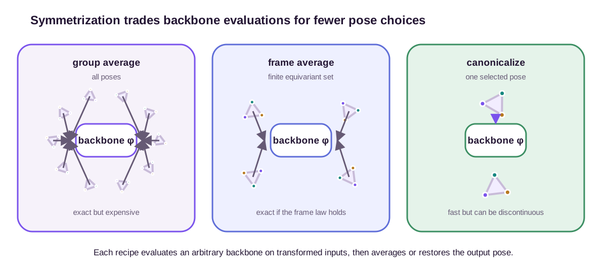
The four-pose backbone separates the recipes numerically. Define the canonical pose of \(x\) to be \(e\), and define a two-pose frame \(\mathcal F(x)=\{e,u^2\}\). On a transformed input, both choices must move with the input:
\[h(u^j\!\cdot x)=u^j, \qquad \mathcal F(u^j\!\cdot x) =\{u^j,u^{j+2}\}.\]Then canonicalization always feeds \(x\) to the backbone and returns \(2\). The two-pose frame average always returns \((2-2)/2=0\). Full group averaging returns \(4\). A one-sample Monte Carlo average returns one of \(\{2,6,-2,10\}\). All four wrappers use the same backbone and input orbit, yet they define different invariant functions:
| wrapper | value on the orbit | backbone evaluations | guarantee |
|---|---|---|---|
| one canonical pose | 2 | 1 | exact if the single pose law holds |
| two-pose frame | 0 | 2 | exact if the whole set law holds |
| full \(C_4\) average | 4 | 4 | exact \(C_4\) invariance |
| Monte Carlo from \(C_4\) | random | \(M\) | exact in expectation; finite-sample guarantee depends on coupling |
There is no reason for the three deterministic values to agree. Canonicalization, frame averaging, and group averaging coincide only when the backbone already gives compatible values on the poses that one method discards and another retains. Their shared symmetry guarantee does not make them the same projection of an arbitrary backbone.
Frame averaging resolves a finite sign ambiguity but not every degeneracy. When PCA eigenvalues repeat, the admissible bases form a continuous family inside the repeated eigenspace. Selecting a finite subset can still jump under small perturbations. Exact equivariance at each input does not guarantee that the averaged network is continuous across these jumps.
The stabilizer condition is a useful implementation test. For every \(s\in G_x\), a valid frame must satisfy \(\mathcal F(x)=s\mathcal F(x)\) because \(s\cdot x=x\). If a code path returns one PCA sign at a symmetric input, this equality fails before the backbone is evaluated. Random tie-breaking does not repair the set law; it changes the claim from deterministic equivariance to a probabilistic one that needs its own coupling analysis.
The number of evaluations is also direct computational overhead. A three-dimensional PCA frame with all sign combinations requires eight backbone passes for \(O(3)\). Sampling one frame reduces the cost to one pass, as stochastic frame-averaging models do, but introduces estimator variance. Symmetry may then hold in expectation or in distribution rather than for every finite random draw.
Probabilistic symmetrization makes the frame weighted
Canonicalization, finite frame averaging, and group averaging can be written with one conditional distribution over poses. Let \(q(dg\mid x)\) be a probability measure on \(G\) that transforms by pushforward:
\[q(\,\cdot\mid h\cdot x)=h_{\#}q(\,\cdot\mid x).\]This means that transforming the input by \(h\) left-multiplies every sampled pose by \(h\). The symmetrized function is
\[F_q(x) =\mathbb{E}_{g\sim q(\cdot\mid x)} \left[ \rho_Y(g)\phi(g^{-1}\cdot x) \right].\]A point mass at one equivariant pose gives deterministic canonicalization. A uniform distribution on a finite frame gives frame averaging. Haar measure gives group averaging. A learned weighted distribution gives probabilistic symmetrization.
The pushforward law automatically audits stabilizers. If \(s\in G_x\), then \(s\cdot x=x\) and hence
\[q(\,\cdot\mid x) =q(\,\cdot\mid s\cdot x) =s_{\#}q(\,\cdot\mid x).\]A point mass can satisfy this equality only if its pose is fixed by left multiplication by every stabilizer element, which is impossible for a nontrivial stabilizer. A distribution can satisfy it by spreading mass across the stabilizer orbit.
The anisotropic cross gives a continuous weighted construction. Restrict attention to the four quarter-turn poses and choose a temperature \(\tau>0\). At the axis-aligned input \(X_\varepsilon\), assign
\[\begin{aligned} q_\varepsilon(e)=q_\varepsilon(u^2) &=\frac{1+\tanh(\varepsilon/\tau)}{4},\\ q_\varepsilon(u)=q_\varepsilon(u^3) &=\frac{1-\tanh(\varepsilon/\tau)}{4}. \end{aligned}\]The weights are nonnegative and sum to one. When \(\varepsilon/\tau\) is large and positive, the distribution concentrates on the two signed horizontal frames. For a large negative ratio, it concentrates on the signed vertical frames. At the tie, all four poses receive weight \(1/4\), as the fourfold stabilizer requires. Because \(X_{-\varepsilon}=u\cdot X_\varepsilon\), changing the sign shifts the weights by a quarter turn: \(q_{-\varepsilon}=u_{\#}q_\varepsilon\). The weights vary continuously with \(\varepsilon\), although no single selected pose does. This construction proves continuity for this finite family only; it is not a global continuous canonicalizer.
Kim et al. parameterize the pose distribution with a small equivariant network and train it jointly with an arbitrary backbone (Kim et al., 2023). The distribution can concentrate computation on useful poses instead of weighting every frame equally. Dym et al.’s weighted-frame construction provides a complementary theoretical point: carefully chosen weights can preserve continuity where finite unweighted frames cannot.
Four different guarantees for a sampled wrapper
In practice, draw \(g_1,\ldots,g_M\) independently from \(q(\cdot\mid x)\) and estimate
\[\widehat F_M(x) =\frac{1}{M}\sum_{m=1}^M Y_x(g_m), \qquad Y_x(g)=\rho_Y(g)\phi(g^{-1}\!\cdot x).\]The exact expectation is equivariant. Indeed, for an input transformed by \(h\), couple each new pose as \(g'_m=hg_m\). The pushforward law gives the correct marginal distribution, and each summand obeys
\[\begin{aligned} Y_{h\cdot x}(hg_m) &=\rho_Y(hg_m) \phi((hg_m)^{-1}h\cdot x)\\ &=\rho_Y(h)Y_x(g_m). \end{aligned}\]This identity separates four claims that are often compressed into “the sampled model is equivariant.”
- Exact deterministic or per-sample equivariance. Full group averages and valid finite frame averages satisfy the transformation equation on every evaluation. A Monte Carlo pair also satisfies it for every realized draw when transformed inputs use the coupled poses \(hg_m\).
- Coupled-sample equivariance. The two evaluations share randomness through the group action. Their numerical outputs obey \(\widehat F_M(h\cdot x)=\rho_Y(h)\widehat F_M(x)\) exactly, even though either estimate can differ from the full expectation.
- Equality in distribution. If transformed inputs use independent random poses, then \(\widehat F_M(h\cdot x)\) and \(\rho_Y(h)\widehat F_M(x)\) have the same distribution. They are not generally equal in a particular pair of runs.
- Expectation equivariance. Averaging over sampler randomness gives \(F_q(h\cdot x)=\rho_Y(h)F_q(x)\) exactly. This is the weakest numerical guarantee for a single independently sampled evaluation.
Independent residuals shrink as \(M^{-1/2}\)
The four-pose backbone makes the Monte Carlo residual explicit. For invariant outputs, its random summand takes values \(2,6,-2,10\) uniformly, with mean \(\mu=4\) and variance
\[\sigma^2 =\frac{(2-4)^2+(6-4)^2+(-2-4)^2+(10-4)^2}{4} =20.\]With independent sampling with replacement, \(\operatorname{Var}[\widehat F_M(x)]=20/M\). Evaluate \(x\) and \(u\cdot x\) with independent random draws and define the scalar invariance residual
\[\Delta_M =\widehat F_M(u\cdot x)-\widehat F_M(x).\]The two estimates are independent with the same variance, so
\[\mathbb E[\Delta_M]=0, \qquad \operatorname{Var}(\Delta_M)=\frac{40}{M}, \qquad \sqrt{\mathbb E[\Delta_M^2]}=\sqrt{\frac{40}{M}}.\]The root-mean-square residual is approximately \(6.32\) for \(M=1\), \(3.16\) for \(M=4\), and \(1.58\) for \(M=16\). Coupled poses make \(\Delta_M=0\) for every \(M\), but both coupled estimates still have variance \(20/M\) around the exact mean \(4\). Enumerating all four poses without replacement makes that estimator exact at \(M=4\); the \(20/M\) formula applies to independent sampling with replacement.
More samples therefore reduce integration error at the usual \(M^{-1/2}\) rate, while cost grows linearly in \(M\). Coupling removes the symmetry residual between paired evaluations; it does not remove their common Monte Carlo error relative to the group average.
Universality does not settle efficiency or stability
Symmetrization preserves the functions we care about. The operator \(\mathcal{S}\) is linear and idempotent:
\[\mathcal{S}(a\phi+b\psi) =a\mathcal{S}\phi+b\mathcal{S}\psi, \qquad \mathcal{S}(\mathcal{S}\phi)=\mathcal{S}\phi.\]An already equivariant target \(f^{\star}\) is a fixed point, so \(\mathcal{S}f^{\star}=f^{\star}\). If an unrestricted backbone family can approximate \(f^{\star}\) on a compact domain, symmetrizing that family does not remove the target from its closure. This projection argument is the source of many universality results for averaging and canonicalization.
The approximation statement has assumptions worth keeping visible. Suppose \(\rho_Y(g)\) is orthogonal and the transformed compact domain contains every \(g^{-1}\!\cdot x\) used by the average. Then
\[\begin{aligned} \left\lVert (\mathcal S\phi)(x)-f^\star(x) \right\rVert &=\left\lVert \int_G\rho_Y(g) \left[\phi(g^{-1}\!\cdot x)-f^\star(g^{-1}\!\cdot x)\right] d\mu(g) \right\rVert\\ &\le \sup_{z}\lVert\phi(z)-f^\star(z)\rVert. \end{aligned}\]The equality inserts equivariance of \(f^\star\); the inequality uses the triangle inequality and norm preservation by \(\rho_Y\). Thus group averaging does not enlarge a uniform approximation error. A normalized equivariant pose distribution gives the same fixed-point identity, because each integrand equals \(f^\star(x)\) when \(\phi=f^\star\). It need not be the same linear projection as Haar averaging, and a learned nonuniform distribution can produce a different function for every non-equivariant backbone.
Universality also does not imply continuity. A sufficient route for the weighted construction is that \(x\mapsto q(\cdot\mid x)\) varies weakly continuously and that \((x,g)\mapsto\rho_Y(g)\phi(g^{-1}\!\cdot x)\) is bounded and continuous on the relevant compact set. Then the expectation varies continuously. A hard argmax pose, a discontinuous support change, or a sampler whose weights collapse at a tie can violate those premises. The smooth cross weights above satisfy them on that one-dimensional family; they do not establish them on the full point-cloud space.
Universality says little about the cost of reaching a useful approximation. Group averaging can require many evaluations. Finite frame averaging multiplies backbone cost by the frame size. Deterministic canonicalization is cheap but can hand the backbone a discontinuous canonical target. Local frames are efficient and preserve fine geometric information, but they become singular when the vectors defining a frame are degenerate. Learned and probabilistic frames add parameters and sampling variance while improving adaptability.
The cost is counted in backbone evaluations
Let \(C_\phi\) be the cost of one unrestricted backbone evaluation, \(C_{\mathrm{pose}}\) the cost of constructing a deterministic pose or frame, and \(C_q\) the cost of a learned pose distribution. Let \(K\) be the size of a full finite group or quadrature, \(L\) the frame size, and \(M\) the Monte Carlo sample count. Ignoring inexpensive rigid transformations, the inference costs are approximately
\[\begin{array}{ll} \text{canonicalization:}&C_{\mathrm{pose}}+C_\phi,\\ \text{full group or quadrature:}&K C_\phi,\\ \text{finite frame:}&C_{\mathrm{pose}}+L C_\phi,\\ \text{probabilistic Monte Carlo:}&C_q+M C_\phi. \end{array}\]For the four-pose table, these are one, four, two, and \(M\) backbone passes, respectively. Parallel evaluation reduces latency if memory can hold \(K\) or \(L\) transformed batches, but it does not reduce floating-point work. Serial evaluation keeps activation memory near one pass but multiplies latency. During training, retaining every pose’s activations can multiply backbone memory as well as compute; checkpointing or sequential accumulation trades memory back for more work.
The pose mechanism has its own conditioning cost. For PCA, perturbation bounds scale inversely with the eigengap. The cross has gap \(\lvert\varepsilon\rvert\), so a covariance perturbation of norm \(\delta\) can rotate the principal subspace by order \(\delta/\lvert\varepsilon\rvert\) away from the exact tie. Local Gram–Schmidt has the analogous denominator \(\lvert\sin\theta\rvert\). Increasing backbone capacity does not repair either geometric condition number.
Sampling introduces a separate accuracy budget. To halve the root-mean-square Monte Carlo error, one needs roughly four times as many independent samples. A learned \(q\) may reduce variance by concentrating on poses where the integrand varies less, but it changes the weighting unless its objective preserves the desired target. Equivariance of the pushforward distribution does not imply unbiasedness with respect to Haar group averaging. One must decide whether the intended operator is the learned weighted expectation or an importance-weighted estimate of Haar integration.
The practical choice is therefore governed by the geometry of the ambiguous inputs. If degeneracies are excluded by construction, one stable local frame may be enough. If a small finite ambiguity such as eigenvector signs dominates, frame averaging is attractive. If symmetric configurations are common or near-symmetries matter physically, a weighted or probabilistic frame can trade several evaluations for smoother behavior. A built-in equivariant architecture remains preferable when exact symmetry at every evaluation and predictable runtime matter more than reusing an unrestricted backbone.
| regime | ambiguity or geometry | guarantee at inference | stability obligation | backbone evaluations | sensible choice |
|---|---|---|---|---|---|
| deterministic canonical pose | unique pose with a gap bounded away from zero | exact per evaluation if the pose law holds | canonicalizer must be continuous enough for the task | 1 | reuse a large unrestricted backbone when degeneracies are excluded |
| local frame | reliable non-collinear local vectors | exact \(SO(3)\) scalarization/vectorization locally | control small norms, collinearity, frame transitions, and parity | usually 1 | directional message passing with stable geometric anchors |
| finite equivariant frame | finite sign or permutation ambiguity | exact per evaluation if the set law holds | support must close under every stabilizer; continuity is separate | \(L\) | PCA signs or a small known ambiguity |
| full finite group | genuinely finite symmetry group | exact per evaluation for that group | no pose selector; does not cover a larger continuous group | \(K=\lvert G\rvert\) | small groups and unrestricted backbones |
| weighted or Monte Carlo poses | continuous or data-dependent ambiguity | expectation exact; coupled samples exact; independent samples equal in distribution | pushforward law, weight continuity, and variance control | \(M\) | flexible reuse when approximate runtime is acceptable |
| built-in equivariant layers | symmetry needed at every internal stage | exact per evaluation up to numerical arithmetic | each primitive must respect its representation law | 1 | predictable runtime, many repeated evaluations, or force-sensitive models |
No row dominates the others. The one-pass methods put more structure into the pose mechanism or the backbone. The averaging methods buy architecture independence with repeated evaluations. A regime should be selected by the symmetry level the application actually tests: deterministic equality, paired equality under controlled randomness, equality of output laws, or equality only after averaging many runs.
Frames do not eliminate the work of equivariant design. They concentrate it in the pose mechanism. The quotient view tells us what should be forgotten, local frames tell us how to express geometry without forgetting it, and symmetrization tells us how to make an arbitrary function respect the group. The discontinuities reveal the price of asking one coordinate system to represent a space in which some objects have no unique orientation.
References
- Du, W., Zhang, H., Du, Y., Meng, Q., Chen, W., Zheng, N., Shao, B., & Liu, T.-Y. (2022). SE(3) equivariant graph neural networks with complete local frames. Proceedings of the 39th International Conference on Machine Learning, 5583–5608. ↩
- Puny, O., Atzmon, M., Smith, E. J., Misra, I., Grover, A., Ben-Hamu, H., & Lipman, Y. (2022). Frame averaging for invariant and equivariant network design. International Conference on Learning Representations. ↩
- Kaba, S.-O., Mondal, A. K., Zhang, Y., Bengio, Y., & Ravanbakhsh, S. (2023). Equivariance with learned canonicalization functions. Proceedings of the 40th International Conference on Machine Learning, 15546–15566. ↩
- Kim, J., Nguyen, T. D., Suleymanzade, A., An, H., & Hong, S. (2023). Learning probabilistic symmetrization for architecture agnostic equivariance. Advances in Neural Information Processing Systems, 36. ↩
- Dym, N., Lawrence, H., & Siegel, J. W. (2024). Equivariant frames and the impossibility of continuous canonicalization. Proceedings of the 41st International Conference on Machine Learning, 12228–12267. ↩