On this page
Adapted from my 2025 Machine Learning for Molecules and Geometric Deep Learning lectures. Symmetry is only the beginning: a simulation-ready potential must also be conservative, smooth, scalable, and reliable on the configurations it will visit. The spherical-layers and tensor-product chapters develop the typed operations used here.
Attention has an appealing interpretation for atomistic systems: an atom should decide which neighbors matter before combining what they say. Geometry makes that sentence harder than it sounds. A Transformer’s attention weight is a scalar, while its hidden features may be vectors and higher-order spherical tensors. An arbitrary query–key comparison can silently destroy rotation equivariance.
The resolution is a useful design principle: routing must be invariant, while content may be equivariant. Queries and keys are built as typed geometric features, but their compatibility is reduced to an invariant scalar. That scalar can safely modulate an equivariant value. This principle connects the SE(3)-Transformer to Equiformer and its descendants. The principle is necessary, but it is not yet a layer: normalization, residual paths, gates, aggregation, and readout must obey the same typing rules.
Yet a model that respects rotations is not automatically a good interatomic potential. Molecular dynamics asks for more: a scalar energy that is extensive, forces that are derivatives of that energy, smooth behavior as neighbors cross a cutoff, enough range to capture the relevant physics, and low enough cost to evaluate for millions of time steps. The real design problem begins where equivariance ends.
Attention has to respect feature types
From a legal score to a complete block
Let atom \(i\) carry a collection of spherical features
\[\mathbf{h}_i = \bigoplus_{\ell=0}^{L} \mathbf{h}_i^{(\ell)}, \qquad \mathbf{h}_i^{(\ell)} \mapsto \mathbf{D}^{(\ell)}(\mathbf{R}) \mathbf{h}_i^{(\ell)}\]under a rotation \(\mathbf{R}\in SO(3)\). Type \(\ell=0\) features are scalars, type \(\ell=1\) features rotate as vectors, and higher types carry finer angular structure. The relative position
\[\mathbf{r}_{ij}=\mathbf{r}_j-\mathbf{r}_i\]removes global translation. Radial functions of \(r_{ij}=\lVert\mathbf{r}_{ij}\rVert\) and spherical harmonics of \(\widehat{\mathbf{r}}_{ij}\) then provide invariant and equivariant edge information.
Ordinary dot-product attention begins with queries, keys, and values. The geometric version keeps the same roles, but every object has a type. Suppressing multiplicity-channel indices, write
\[\begin{aligned} \mathbf{q}_i^{(\ell)} &= \mathbf{W}_Q^{(\ell)}\mathbf{h}_i^{(\ell)},\\ \mathbf{k}_{ij}^{(\ell)} &= \Phi_K^{(\ell)} \left(\mathbf{h}_j, r_{ij}, \mathbf{Y}(\widehat{\mathbf{r}}_{ij})\right),\\ \mathbf{v}_{ij}^{(\ell)} &= \Phi_V^{(\ell)} \left(\mathbf{h}_j, r_{ij}, \mathbf{Y}(\widehat{\mathbf{r}}_{ij})\right). \end{aligned}\]Here \(\Phi_K\) and \(\Phi_V\) are equivariant maps, typically assembled from tensor products, radial networks, and type-preserving linear layers. Under rotation, each query, key, and value block transforms through the same \(\mathbf{D}^{(\ell)}(\mathbf{R})\) associated with its type. The detailed Clebsch–Gordan construction belongs in the tensor-product chapter linked above. What matters at this interface is that the maps advertise and satisfy a transformation law.
Normalization already requires care. A component-wise normalization of a vector can depend on the coordinate frame. A safe alternative normalizes a whole irrep block by an invariant magnitude,
\[\overline{\mathbf{q}}_i^{(\ell)} = \frac{\mathbf{q}_i^{(\ell)}} {\sqrt{\lVert\mathbf{q}_i^{(\ell)}\rVert^2+\epsilon}}, \qquad \overline{\mathbf{k}}_{ij}^{(\ell)} = \frac{\mathbf{k}_{ij}^{(\ell)}} {\sqrt{\lVert\mathbf{k}_{ij}^{(\ell)}\rVert^2+\epsilon}}.\]The denominators are scalars, so the normalized blocks retain their types. In a model with several copies of each irrep, learned linear maps and normalization statistics may mix multiplicity channels, but they must act identically across the magnetic components of a single irrep. This is the same restriction derived from Schur’s lemma in the tensor-product post.
The attention logit must not transform at all. One valid construction is
\[s_{ij} = \sum_{\ell=0}^{L} \frac{1}{\sqrt{d_\ell}} \left\langle \overline{\mathbf{q}}_i^{(\ell)}, \overline{\mathbf{k}}_{ij}^{(\ell)} \right\rangle, \qquad \alpha_{ij} = \frac{\exp(s_{ij})} {\sum_{k\in\mathcal{N}(i)}\exp(s_{ik})}.\]In a real orthonormal irrep basis, Wigner matrices are orthogonal. Therefore
\[\left\langle \mathbf{D}^{(\ell)}(\mathbf{R})\mathbf{q}, \mathbf{D}^{(\ell)}(\mathbf{R})\mathbf{k} \right\rangle = \mathbf{q}^{\mathsf T} \mathbf{D}^{(\ell)}(\mathbf{R})^{\mathsf T} \mathbf{D}^{(\ell)}(\mathbf{R}) \mathbf{k} = \langle\mathbf{q},\mathbf{k}\rangle.\]The logits and softmax weights are invariant. Softmax does not create equivariance; it merely preserves the invariance of its scalar inputs. The value aggregation
\[\mathbf{m}_i^{(\ell)} = \sum_{j\in\mathcal{N}(i)} \alpha_{ij}\mathbf{v}_{ij}^{(\ell)}\]is consequently equivariant: multiplying a rotating feature by an invariant scalar changes its magnitude, not its transformation law.
The aggregation must now pass through the rest of a Transformer block. A type-preserving output map and residual connection give
\[\widetilde{\mathbf{h}}_i^{(\ell)} = \mathbf{h}_i^{(\ell)} + \mathbf{W}_O^{(\ell)}\mathbf{m}_i^{(\ell)}.\]The addition is legal because both summands have the same type. For \(\ell>0\), an invariant gate supplies a safe nonlinearity,
\[g_i^{(\ell)} = \sigma\!\left(a_i^{(\ell)}\right), \qquad \mathbf{h}_i^{(\ell),+} = g_i^{(\ell)}\widetilde{\mathbf{h}}_i^{(\ell)},\]where the gate logit \(a_i^{(\ell)}\) is type \(0\). Scalar channels may use ordinary scalar activations. Applying ReLU independently to the Cartesian components of a vector is not safe: rotating first and thresholding generally differs from thresholding first and rotating.
For a potential, the final readout uses only scalar channels:
\[\varepsilon_i = \mathbf{w}_E^{\mathsf T}\mathbf{h}_i^{(0),+}, \qquad E_\theta = \sum_i \varepsilon_i.\]This completes the proof by composition. Equivariant maps create typed keys and values; invariant contractions create logits; scalar softmax weights route values; same-type residuals preserve the representation; scalar gates modulate nonscalars; and a scalar sum returns invariant energy. A single illegal normalization or component-wise nonlinearity would break that chain even if the attention equation itself were correct.
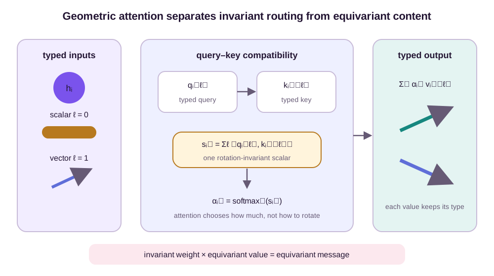
This is the essential move in the SE(3)-Transformer (Fuchs et al., 2020). The architecture is more elaborate than these equations—its keys and values are steerable convolutions—but its attention proof reduces to the same sentence: invariant weights modulate equivariant values. The full block needs the longer closure argument above.
A worked rotation example
The invariance of a typed inner product is easiest to see for type-1 features. Take a two-dimensional slice of three-dimensional space and set
\[\mathbf{q}=\begin{bmatrix}1\\0\end{bmatrix}, \qquad \mathbf{k}_1=\begin{bmatrix}1\\0\end{bmatrix}, \qquad \mathbf{k}_2=\begin{bmatrix}0\\1\end{bmatrix}.\]The logits are \(s_1=1\) and \(s_2=0\), so
\[(\alpha_1,\alpha_2) = \operatorname{softmax}(1,0) \approx (0.73,0.27).\]Now rotate everything by \(90^\circ\) with
\[\mathbf{R} = \begin{bmatrix}0&-1\\1&0\end{bmatrix}.\]The query and keys change direction, but
\[(\mathbf{R}\mathbf{q})^{\mathsf T} (\mathbf{R}\mathbf{k}_a) = \mathbf{q}^{\mathsf T}\mathbf{k}_a\]for either key \(a\). The attention weights stay at \((0.73,0.27)\). To verify the value path rather than stopping at the scores, choose
\[\mathbf{v}_1= \begin{bmatrix}2\\1\end{bmatrix}, \qquad \mathbf{v}_2= \begin{bmatrix}-1\\3\end{bmatrix}.\]The output before its type-preserving linear map is
\[\mathbf{m} = 0.731\mathbf{v}_1+0.269\mathbf{v}_2 = \begin{bmatrix}1.193\\1.538\end{bmatrix}.\]After the same rotation, the two values become \(\mathbf{R}\mathbf{v}_1=(-1,2)^{\mathsf T}\) and \(\mathbf{R}\mathbf{v}_2=(-3,-1)^{\mathsf T}\). The recomputed output is
\[\begin{aligned} \mathbf{m}' &= 0.731 \begin{bmatrix}-1\\2\end{bmatrix} + 0.269 \begin{bmatrix}-3\\-1\end{bmatrix}\\ &= \begin{bmatrix}-1.538\\1.193\end{bmatrix} = \mathbf{R}\mathbf{m}. \end{aligned}\]This equality is the operational definition of equivariance: the output computed from rotated inputs equals the rotated original output. It is stronger than saying that the attention weights did not change. The weights encode the same relational choice, while the transported geometric content follows the frame.
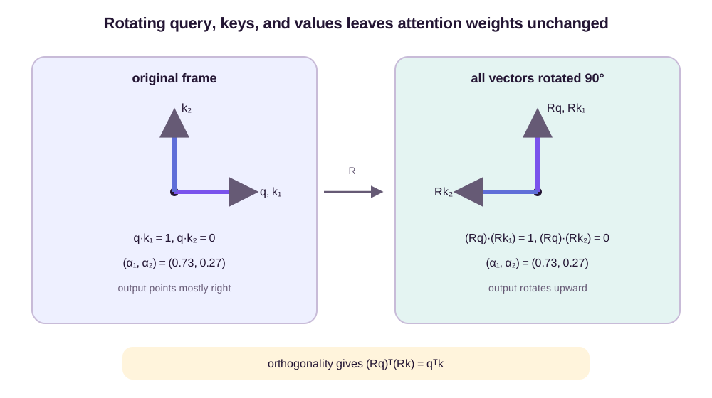
Inner-product attention is not the only possibility. Equiformer generates attention logits with an invariant nonlinear network after equivariant tensor-product processing, which gives the scoring function more freedom than a single dot product (Liao & Smidt, 2023). The non-negotiable requirement is not a particular formula; it is that the final logit belongs to type \(0\). A nonlinear score may change the numerical weights in this example, but it must reproduce the same weights after jointly rotating query, keys, values, and edges.
Architectures differ in where they spend geometric computation
Architecture names are useful only after fixing the contract. Consider a controlled local potential with the following interface: atoms and coordinates enter; a radius graph supplies at most \(k\) neighbors per atom; hidden features contain types \(\ell=0,1,2\); every block preserves equivariance; and the final output is an invariant atomic energy whose coordinate gradient supplies forces. Hold the channel budget, cutoff, and number of interaction blocks fixed. Three choices remain genuinely different.
First, routing may be a fixed neighbor sum or invariant attention. Attention can amplify one chemically relevant neighbor and suppress another at the same distance, but it does not enlarge the cutoff or create a new tensor type. Second, angular coupling may use full \(SO(3)\) tensor products or rotate each edge into a canonical axis and exploit the residual \(SO(2)\) structure. This changes computational organization, not the transformation law promised at the interface. Third, correlation order may emerge through repeated pairwise messages or be exposed explicitly by coupling several neighbor densities around a center.
Under this contract, representative architectures locate their geometric computation in different places:
| Controlled choice | Representative construction | What changes | What does not change |
|---|---|---|---|
| Neighbor routing | SE(3)-Transformer / Equiformer attention | Data-dependent invariant weights | Cutoff, tensor types, and scalar-energy requirement |
| Angular basis evaluation | Full \(SO(3)\) or eSCN-style edge-aligned \(SO(2)\) coupling | Number and sparsity of angular contractions | Equivariant input-output law |
| Local correlation | Pairwise messages or MACE-style higher-order products | How directly multiple neighbors interact | Locality radius and invariant readout |
The SE(3)-Transformer starts from steerable convolutions and adds data-dependent invariant attention. It supplies the conceptual template used above: values carry geometry and scalar weights select neighbors. Equiformer recasts more of the Transformer stack—attention, normalization, and feed-forward updates—as typed operations. EquiformerV2 then incorporates edge alignment and revised normalization to scale higher-degree representations (Liao et al., 2024). These changes matter even when the external energy-and-force contract is identical.
The key efficiency result behind eSCN is geometric rather than a learned approximation. Align the local coordinate axis with an edge, perform coupling in that frame, and exploit the fact that rotations about the edge preserve magnetic index structure. For the relevant tensor products, Passaro and Zitnick reduce the leading dependence on maximum degree from \(O(L^6)\) to \(O(L^3)\) (Passaro & Zitnick, 2023). The asymptotic statement is not a wall-clock prediction: rotations into and out of edge frames, channel mixing, memory movement, and coordinate derivatives remain.
MACE spends capacity on a different axis. It builds higher-correlation equivariant features inspired by the atomic cluster expansion, so one interaction can couple information from several neighbors rather than waiting for higher body order to emerge only through depth (Batatia et al., 2022). Suppose a central atom has neighbors \(j\) and \(k\) and the target contains an angular term \(g(r_{ij},r_{ik},\widehat{\mathbf{r}}_{ij}\cdot\widehat{\mathbf{r}}_{ik})\). A pairwise layer can encode each edge, but their joint dependence must be formed after aggregation or in later processing. A higher-correlation construction exposes that joint term directly. Attention, by contrast, can decide that edge \(ij\) matters more than \(ik\) without automatically representing their joint angle.
This comparison avoids a misleading model catalog. Attention, edge alignment, and higher-order products answer different questions: which neighbor, in which computational frame, and at what correlation order. They can be combined. For Wigner-basis conventions, coupling paths, and broader implementation strategies, see the spherical and tensor-product posts linked in the opening note. Here the criterion is narrower: after any of those internal choices, does the model still produce a differentiable invariant energy at an affordable cost?
Put numbers on the fixed contract
Consider one center with \(k=32\) neighbors and hidden multiplicities \(C_0=64\), \(C_1=32\), and \(C_2=16\). The number of stored scalar components per atom is
\[D = C_0(2\cdot0+1) +C_1(2\cdot1+1) +C_2(2\cdot2+1) =64+96+80 =240.\]This count is an identity for the stated representation, not a runtime model. It already shows why “64 channels” is ambiguous in an equivariant network: a type-2 channel stores five magnetic components. For the center and its 32 neighbors, merely retaining one 240-component float32 value vector per directed edge takes
\[32\times240\times4 =30{,}720\ \text{bytes},\]before queries, keys, coupling intermediates, and gradients. Four attention heads do not necessarily quadruple every tensor—implementations may share values—but they do create four scalar routing weights per edge and often partition or replicate channel work.
Now compare two changes while holding \(k\) and \(D\) fixed. Adding invariant attention requires, at minimum, a score for each of the 32 edges plus a weighted value sum. It changes routing but leaves the 240-component type inventory intact. Raising the angular truncation from \(L=2\) to \(L=3\) with, say, \(C_3=16\) adds
\[C_3(2\cdot3+1)=112\]components per atom, a 47% increase from 240 to 352 even before counting the additional legal coupling paths. That change enriches angular content rather than routing. Replacing full \(SO(3)\) contractions with an edge-aligned implementation may reduce the cost of those paths, but it does not make the 112 output components disappear.
Correlation order creates a third, distinct bill. A pairwise message examines \(O(k)\) edge objects at a center. A literal enumeration of unordered neighbor pairs would expose \(k(k-1)/2=496\) pairs when \(k=32\). MACE-style constructions avoid naively materializing every tuple by forming and contracting aggregated neighbor densities, but their wider products still pay for the requested correlation channels. It would therefore be wrong to infer that one higher-order layer costs exactly 496 times one pairwise layer; the controlled calculation only identifies the combinatorial object being compressed.
These numbers sharpen the architectural tradeoff. Attention can redistribute a fixed edge budget. Higher \(L\) allocates more storage and contractions to directional resolution. Higher correlation order allocates computation to joint neighbor structure. Edge alignment changes how angular contractions are executed. Depth repeats whichever choice was made and expands the graph receptive field only along existing edges. A fair ablation holds the other axes fixed; otherwise an apparent gain from “attention” may actually come from more typed components, a larger cutoff, or a different body-order budget.
A force field is an energy model with derivatives
Extensivity is a modeling contract
For atom types \(\mathbf{Z}=(Z_1,\ldots,Z_N)\) and coordinates \(\mathbf{r}=(\mathbf{r}_1,\ldots,\mathbf{r}_N)\), an interatomic potential approximates a scalar potential-energy surface
\[E_\theta(\mathbf{Z},\mathbf{r}).\]Rigid translations and rotations must leave this scalar unchanged. For systems whose energy is size-extensive, the usual local decomposition is
\[E_\theta(\mathbf{Z},\mathbf{r}) = \sum_{i=1}^{N} \varepsilon_{\theta,i},\]where each atomic contribution is read from the invariant part of atom \(i\)’s final representation. If two subsystems \(A\) and \(B\) have no connecting interaction, the construction gives
\[E_\theta(A\sqcup B) = \sum_{i\in A}\varepsilon_i+ \sum_{i\in B}\varepsilon_i =E_\theta(A)+E_\theta(B).\]Thus two noninteracting copies have twice the energy. This is size extensivity, not a consequence of rotation symmetry. It depends on the additive readout and on the representation making the two components independent. A global normalization over all atoms, for example, could couple disconnected copies and violate the identity. The local sum also permits approximately linear cost in \(N\) when density and neighbor count remain bounded.
Invariant energy makes covariant forces
Forces should be obtained from the same energy:
\[\mathbf{F}_{\theta,i} = -\nabla_{\mathbf{r}_i} E_\theta(\mathbf{Z},\mathbf{r}).\]This one equation enforces several facts at once. Let \(\mathbf{r}'_i=\mathbf{R}\mathbf{r}_i+\mathbf{b}\) with \(\mathbf{R}\in SO(3)\), and assume
\[E_\theta(\mathbf{Z},\mathbf{r}') = E_\theta(\mathbf{Z},\mathbf{r}).\]Because \(\mathbf{r}_i=\mathbf{R}^{\mathsf T}(\mathbf{r}'_i-\mathbf{b})\), the chain rule gives
\[\nabla_{\mathbf{r}'_i}E_\theta(\mathbf{r}') = \mathbf{R}\nabla_{\mathbf{r}_i}E_\theta(\mathbf{r}),\]and hence
\[\mathbf{F}'_{\theta,i} = \mathbf{R}\mathbf{F}_{\theta,i}.\]The scalar energy is invariant, while its gradient is covariant. No separate vector-output argument is needed.
Translation and rotation invariance also impose collective identities. Translate every atom infinitesimally by \(t\mathbf{a}\). Differentiating invariance at \(t=0\) yields
\[0 = \frac{d}{dt}E(\mathbf{r}_1+t\mathbf{a},\ldots,\mathbf{r}_N+t\mathbf{a})\bigg|_{t=0} = \mathbf{a}\cdot\sum_i\nabla_{\mathbf{r}_i}E.\]This holds for every \(\mathbf{a}\), so the total internal force vanishes. For an infinitesimal rotation with angular vector \(\boldsymbol{\omega}\), \(\delta\mathbf{r}_i=\boldsymbol{\omega}\times\mathbf{r}_i\). Then
\[0 = \sum_i \nabla_{\mathbf{r}_i}E\cdot (\boldsymbol{\omega}\times\mathbf{r}_i) = -\boldsymbol{\omega}\cdot \sum_i\mathbf{r}_i\times\mathbf{F}_i.\]Since this is true for every \(\boldsymbol{\omega}\),
\[\sum_i \mathbf{F}_{\theta,i}=\mathbf{0}, \qquad \sum_i \mathbf{r}_i\times\mathbf{F}_{\theta,i}=\mathbf{0}.\]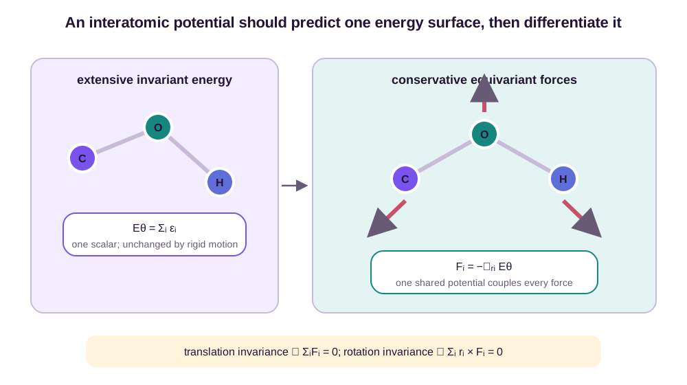
These identities assume an isolated system with no external field. Periodic cells, fixed constraints, applied fields, and driven boundaries require the corresponding qualified statement. They also say nothing about accuracy: an invariant but wrong energy produces perfectly covariant but wrong forces.
Equivariance does not imply conservativity
A direct vector head can be equivariant, translation invariant, torque balanced, and still not be conservative. Consider three atoms and the relative vectors
\[\mathbf{q}=\mathbf{r}_2-\mathbf{r}_1, \qquad \mathbf{p}=\mathbf{r}_3-\mathbf{r}_1, \qquad a=\mathbf{q}^{\mathsf T}\mathbf{p}.\]Define a direct force head by
\[\mathbf{F}_2=a\mathbf{q}, \qquad \mathbf{F}_3=\mathbf{0}, \qquad \mathbf{F}_1=-a\mathbf{q}.\]Translation leaves \(\mathbf{q}\) and \(\mathbf{p}\) unchanged. Under any three-dimensional rotation \(\mathbf{R}\), the scalar \(a\) is invariant and \(\mathbf{q}\) rotates, so every force obeys \(\mathbf{F}_i' = \mathbf{R}\mathbf{F}_i\). The net force is exactly zero. Taking atom 1 as the torque origin also gives
\[\boldsymbol{\tau} = \mathbf{q}\times\mathbf{F}_2 + \mathbf{p}\times\mathbf{F}_3 = a\,\mathbf{q}\times\mathbf{q} = \mathbf{0}.\]Nevertheless, suppose a scalar \(E(\mathbf{q},\mathbf{p})\) generated these forces. Because \(\mathbf{F}_2=-\partial E/\partial\mathbf{q}\) and \(\mathbf{F}_3=-\partial E/\partial\mathbf{p}\), it would have to satisfy
\[\frac{\partial E}{\partial\mathbf{q}} = -a\mathbf{q}, \qquad \frac{\partial E}{\partial\mathbf{p}} = \mathbf{0}.\]For a twice-differentiable scalar, the two mixed derivative blocks must be transposes of one another. Here
\[\frac{\partial}{\partial\mathbf{p}} \left(-a\mathbf{q}\right) = -\mathbf{q}\mathbf{q}^{\mathsf T}, \qquad \frac{\partial}{\partial\mathbf{q}} \left(\mathbf{0}\right) = \mathbf{0}.\]They disagree whenever \(\mathbf{q}\neq\mathbf{0}\). The sign can also be checked from atom 1: \(-\partial E/\partial\mathbf{r}_1=\partial E/\partial\mathbf{q}+\partial E/\partial\mathbf{p}=-a\mathbf{q}=\mathbf{F}_1\), so the contradiction is not caused by mishandling the relative coordinates.
This atomistic witness separates the properties sharply: rotational equivariance, translation invariance, zero net force, and zero torque still do not imply integrability in configuration space. Around any closed path \(\mathcal{C}\), an energy-derived force satisfies
\[\oint_{\mathcal{C}} \sum_i \mathbf{F}_{\theta,i}\cdot d\mathbf{r}_i =0,\]whereas a direct force model has no reason to do so. Direct-force models can still be useful when force accuracy or speed dominates and the application tolerates a nonconservative field. But that choice changes the physical contract and must be evaluated as such.
Energy-derived forces are not sufficient by themselves. A conservative continuous-time vector field can still show numerical energy drift under a coarse or nonsymplectic integrator. Conversely, reducing the time step can hide an integration error but cannot repair the wrong potential surface. Fu et al. show that low held-out errors need not predict stable downstream simulations and identify smoothness choices that materially affect energy conservation (Fu et al., 2025). The derivative behavior of the learned surface matters, not merely its values on test structures. The downstream numerical issues are developed more fully in the post on molecular dynamics and enhanced sampling.
Force supervision constrains the shape of the surface
Values locate the surface; forces tilt it
A practical objective combines energies and forces:
\[\mathcal{L}(\theta) = \lambda_E \left(E_\theta-E^\star\right)^2 + \frac{\lambda_F}{N} \sum_{i=1}^{N} \left\lVert -\nabla_{\mathbf{r}_i}E_\theta -\mathbf{F}_i^\star \right\rVert^2.\]One energy label constrains one scalar value. A force-labeled configuration provides up to \(3N\) derivative components, revealing the local slope of the potential-energy surface. The components are not all statistically independent—translation and rotation identities introduce structure—but they are far richer local information than one scalar. This is why force training can be extremely data-efficient. It is also why training is expensive: differentiating a force loss with respect to parameters requires mixed second derivatives, \(\partial^2E_\theta/(\partial\theta\,\partial\mathbf{r})\).
Consider a stretched diatomic molecule with distance \(r\). Near equilibrium \(r_0\), a harmonic approximation is
\[E(r)=E_0+\frac{k}{2}(r-r_0)^2, \qquad F_r=-\frac{dE}{dr}=-k(r-r_0).\]An energy sample at \(r_0\) fixes the minimum value but says nothing about curvature \(k\). Make the ambiguity numerical. Set \(r_0=1.0\ \text{\AA}\) and \(E_0=0\), and consider two candidate surfaces,
\[E_1(r)=\frac{1}{2}(r-1)^2, \qquad E_4(r)=\frac{4}{2}(r-1)^2,\]with energy in eV and distance in angstroms. Both match the equilibrium energy exactly. At \(r=1.1\ \text{\AA}\), however,
\[\begin{array}{c|cc} & E(1.1)\;[\mathrm{eV}] & F_r(1.1)\;[\mathrm{eV}/\text{\AA}]\\ \hline k=1 & 0.005 & -0.1\\ k=4 & 0.020 & -0.4 \end{array}\]Suppose the reference force is \(-0.4\ \mathrm{eV}/\text{\AA}\). The equilibrium energy label leaves the entire line \(E_0=0\) in the \((E_0,k)\) parameter plane feasible; the displaced force label intersects it at \(k=4\). A second energy at \(1.1\ \text{\AA}\) would also identify \(k\) in this exact quadratic model, but the energy separation between the candidates is only \(0.015\) eV while their force separation is \(0.3\ \mathrm{eV}/\text{\AA}\). Force supervision measures the slope directly rather than inferring it from a small difference between two absolute energies.
A force at \(r=0.9\ \text{\AA}\) supplies the complementary value \(+0.4\ \mathrm{eV}/\text{\AA}\) and verifies that the stationary point is a minimum rather than merely a zero crossing on one side. In a many-atom system, the same local picture becomes a Hessian: displacement along normal mode \(\mathbf{u}_a\) produces, to first order,
\[\Delta\mathbf{F} \approx -\mathbf{H}\mathbf{u}_a\,\delta, \qquad \mathbf{H}=\nabla_{\mathbf{r}}^2E.\]Thus nearby force labels reveal curvature along many coordinate directions. They do not, however, determine distant barriers or disconnected basins. A dense cloud around one minimum can yield excellent force error and still say almost nothing about bond breaking.
The loss weights carry units and a sampling choice
The coefficients \(\lambda_E\) and \(\lambda_F\) are not innocent hyperparameters. Energy residuals have units of energy; force residuals have units of energy per length; their raw squared magnitudes also scale differently with system size. Dividing the force sum by \(N\) makes configurations more comparable, but it does not decide whether a rare transition state should matter as much as a thousand equilibrium frames. The empirical loss approximates an integral over the training distribution, not over every configuration a simulation might visit.
For this reason, reporting only a combined loss conceals the learned surface. Energy MAE tests vertical placement, force MAE tests local slopes, and vibrational frequencies or Hessian-vector products probe curvature. Barrier heights, dissociation curves, stress, and virials require their own labels or evaluations. Force supervision supplies a dense local differential signal; it is not a substitute for coverage.
Cutoffs turn locality into a smoothness problem
A cutoff is part of the differentiable model
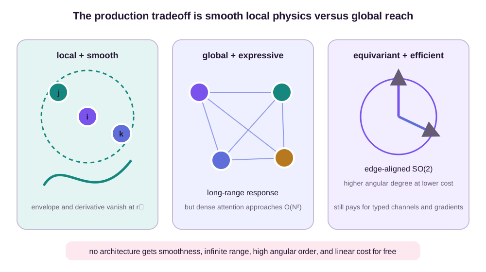
Most scalable potentials build a neighbor graph with cutoff radius \(r_c\). The local environment is finite, and for fixed density the number of edges grows approximately linearly with the number of atoms. A hard cutoff, however, creates a discontinuity when a pair crosses \(r_c\). Even if energy itself is continuous, a nonzero slope at the boundary creates a force jump.
Let an edge contribution be
\[\widetilde{\phi}(r) = s(r)\phi(r),\]where the envelope satisfies
\[s(r_c)=0, \qquad s'(r_c)=0.\]Then both the contribution and its first derivative vanish smoothly as the edge disappears. A useful explicit choice is the quintic envelope
\[s(r) = \begin{cases} 1-10x^3+15x^4-6x^5, & 0\leq x<1,\\ 0, & x\geq 1, \end{cases} \qquad x=\frac{r}{r_c}.\]Direct substitution gives \(s(1)=s'(1)=s''(1)=0\). If \(\phi\) is bounded and twice continuously differentiable near \(r_c\), then
\[\widetilde{\phi}'=s'\phi+s\phi', \qquad \widetilde{\phi}''=s''\phi+2s'\phi'+s\phi''\]both approach zero at the boundary. Extending \(\widetilde{\phi}\) by zero beyond \(r_c\) is therefore \(C^2\). The energy, force, and this edge’s Hessian contribution join continuously. This is a sufficient local regularity statement under the stated assumptions; it does not prove that the whole network has bounded higher derivatives.
Attention adds a subtlety. Multiplying only the value by \(s(r_{ij})\) does not necessarily make the discrete softmax smooth: deleting a neighbor also removes its term from the denominator and can renormalize every surviving value. A smooth local form instead gates the unnormalized weight,
\[w_{ij} = s(r_{ij})\exp(s_{ij}), \qquad \alpha_{ij} = \frac{w_{ij}} {w_{i,\mathrm{self}}+\sum_k w_{ik}},\]with a positive self or baseline weight. As \(r_{ij}\to r_c\), both the disappearing message and its effect on the denominator vanish with the envelope. The precise implementation can differ, but every route through which an edge affects the output must become smooth. The envelope is not cosmetic windowing; it is part of the differentiable architecture.
Neighbor-list algorithms usually maintain a larger skin radius so that the list need not be rebuilt at every time step. The skin improves bookkeeping efficiency; it does not replace the physical cutoff envelope. An interaction may enter the cached list discontinuously without affecting the energy if its gated contribution is still exactly zero outside \(r_c\).
A controlled locality counterexample
Locality also limits physical reach. Consider two isolated point charges, \(+e\) and \(-e\), separated in vacuum by \(R\), with a local model cutoff \(r_c=5\ \text{\AA}\). For every \(R>r_c\) the radius graph has two disconnected one-atom components. A strictly local additive model must return the same energy for \(R=6\ \text{\AA}\) and \(R=8\ \text{\AA}\) because its inputs are identical: two isolated atomic environments.
The Coulomb interaction does not agree. Using \(e^2/(4\pi\epsilon_0)\approx14.4\ \mathrm{eV\,\text{\AA}}\),
\[E_{\mathrm{C}}(R) = -\frac{14.4}{R}\ \mathrm{eV}, \qquad \lvert F_{\mathrm{C}}(R)\rvert = \frac{14.4}{R^2}\ \mathrm{eV}/\text{\AA}.\]At \(6\ \text{\AA}\) the interaction is \(-2.4\) eV with force magnitude \(0.40\ \mathrm{eV}/\text{\AA}\); at \(8\ \text{\AA}\) it is \(-1.8\) eV with force magnitude \(0.225\ \mathrm{eV}/\text{\AA}\). The local model predicts zero change and zero interfragment force in both cases. No additional depth repairs this example because there is no path through vacuum along which a message can travel. Neutral fragments give a less dramatic but analogous dispersion tail, proportional asymptotically to \(-C_6/R^6\).
This is a representation impossibility, not an optimization failure. Covalent bonding and short-range repulsion may be well represented inside a moderate cutoff, but electrostatics, dispersion, charge transfer, and collective response can extend farther. In condensed matter, deeper local message passing can transmit information through intervening atoms, yet that mediated path is not automatically the correct long-range Green’s function. Practical potentials add explicit electrostatic or dispersion terms, charge equilibration, hierarchical propagation, reciprocal-space components, or other local–global hybrids.
Sparse and global attention have different arithmetic
The asymptotic distinction becomes concrete quickly. Take \(N=10{,}000\) atoms and an average of \(k=64\) directed neighbors. Local attention scores
\[M_{\mathrm{local}}=Nk=640{,}000\]edges. Dense global attention scores \(N^2=100{,}000{,}000\) ordered pairs, a factor of
\[\frac{N^2}{Nk}=\frac{N}{k}=156.25\]more. Storing one float32 logit per edge requires about \(2.56\) MB locally and \(400\) MB globally. With eight heads, logits alone occupy roughly \(20.5\) MB versus \(3.2\) GB, before values, typed features, activations, gradients, and neighbor metadata. These figures are arithmetic estimates, not benchmark timings; kernel fusion and hardware utilization can change wall-clock ratios.
Typed geometric values add another axis. Raising \(L\) increases the number of magnetic components and allowed tensor-product paths, while force training retains an autograd graph through coordinates. An edge-aligned \(SO(2)\) kernel can reduce angular contraction cost without changing the \(Nk\) edge count. Sparse attention changes the edge count without eliminating angular work. The two savings are complementary.
Fully global attention restores direct reach at quadratic pair cost. Sparse neighborhoods retain near-linear scaling at fixed density, but they impose the locality counterexample above. A hybrid is justified when its added long-range term targets a known missing interaction, not merely because “global” sounds more expressive.
What equivariance buys—and what it does not
Symmetry removes redundant freedom
Equivariance ties together every rotated copy of a configuration. A model trained on one orientation already knows how its internal vectors and predicted forces should behave in another. NequIP demonstrated the resulting data efficiency for interatomic potentials (Batzner et al., 2022). Equivariant attention adds adaptive neighbor selection without giving up that guarantee.
But equivariance is a constraint, not a complete account of the physics. It removes the need to relearn rotated copies and forbids transformation-inconsistent functions. It does not determine the cutoff, resolve missing long-range interactions, ensure conservative direct-force predictions, prevent extrapolation into untrained chemistry, or make high-degree tensor products cheap. A scalar-only model trained on vast and diverse data can outperform a small equivariant model on some benchmarks; an accurate equivariant model can still produce unstable dynamics if its cutoff is nonsmooth.
The distinction can be stated statistically. Let \(\mathcal{F}\) be a broad hypothesis class and \(\mathcal{F}_{\mathrm{eq}}\subset\mathcal{F}\) its exactly equivariant subset. If the true target obeys the symmetry, restricting to \(\mathcal{F}_{\mathrm{eq}}\) removes functions that fit one orientation but contradict another. That often improves sample efficiency. It does not select the correct member of \(\mathcal{F}_{\mathrm{eq}}\) outside the observed chemical and configurational support. Symmetry reduces variance along group orbits; it does not eliminate extrapolation across bond patterns, charge states, temperatures, or phases.
Turn performance claims into a simulation contract
The right model is therefore chosen against a simulation contract. Each claim needs a matching construction and test:
| Claimed property | Required model or numerical condition | Falsifying evaluation |
|---|---|---|
| Rotation-consistent energies and forces | Invariant energy and equivariant differentiation | Randomly rotate held-out structures and compare transformed outputs to numerical tolerance |
| Conservative internal forces | Forces obtained from one differentiable scalar energy | Closed-loop work or Hessian-symmetry test |
| Size extensivity | Additive contributions with no coupling between disconnected subsystems | Compare one copy with two separated copies |
| Stable NVE dynamics | Smooth potential, conservative forces, suitable integrator, time step, and precision | Energy drift versus trajectory length and time-step refinement |
| Correct equilibrium structure | Accurate energy differences over thermally visited states plus adequate sampling | Radial distributions, populations, free energies, and uncertainty across replicas |
| Correct kinetics | Accurate barriers and curvatures plus an appropriate dynamical model | Transition rates or time correlations, not equilibrium MAE alone |
| Long-range response | Explicit mechanism with the required range and boundary conditions | Separation curves, dielectric response, or system-size scaling |
| Practical throughput | Bounded edge count and affordable typed/derivative computation | End-to-end nanoseconds per atom-step, including neighbor lists and force gradients |
The table separates architectural identities from empirical claims. Exact equivariance can be tested to machine precision; force accuracy and trajectory stability cannot. Energy conservation in continuous time follows from a time-independent differentiable potential, but energy conservation in a numerical trajectory additionally depends on the integrator. Correct equilibrium sampling further depends on whether the learned energy is accurate over the states actually visited and whether the thermostat or sampler explores them.
Return to the harmonic diatomic. The force-trained surface had \(k=4\), while the energy-at-equilibrium-only candidate allowed \(k=1\). For reduced mass \(\mu\), the small-oscillation frequency is
\[\omega=\sqrt{\frac{k}{\mu}}.\]Both potentials are invariant, conservative, smooth, and easy to integrate. Yet the \(k=1\) model predicts half the frequency of the \(k=4\) model. It may produce a numerically stable trajectory with systematically wrong vibrational kinetics. If a trajectory crosses a nonsmooth cutoff, even the correct local curvature does not prevent a force discontinuity. If the forces come from the rotational direct-force witness above, equivariance does not prevent nonzero closed-loop work. Each failure belongs to a different line of the contract.
This is why a single force MAE cannot certify simulation quality. A claim about vibrational spectra calls for Hessians or frequencies. A claim about NVE stability calls for drift curves under time-step refinement. A claim about thermodynamics calls for ensemble observables and free-energy differences. A claim about reactions calls for transition regions and kinetics. The companion post on molecular dynamics and enhanced sampling follows these distinctions from potentials to path distributions; the present chapter stops at the model–simulator boundary.
The deepest connection between equivariant Transformers and machine-learned potentials is not that attention is universally superior. It is that a legal geometric architecture exposes exactly what may be learned freely and what must remain fixed. Attention may learn which interaction matters. Symmetry dictates how its content transforms. The energy construction dictates where forces come from. The cutoff determines which interactions are representable and how derivatives vanish. The simulator determines which empirical errors matter. Smoothness, range, data coverage, and computational scale decide whether those elegant equations survive a real molecular-dynamics run.
References
- Fuchs, F. B., Worrall, D. E., Fischer, V., & Welling, M. (2020). SE(3)-Transformers: 3D Roto-Translation Equivariant Attention Networks. NeurIPS. ↩
- Liao, Y.-L., & Smidt, T. (2023). Equiformer: Equivariant Graph Attention Transformer for 3D Atomistic Graphs. ICLR. ↩
- Liao, Y.-L., Wood, B., Das, A., & Smidt, T. (2024). EquiformerV2: Improved Equivariant Transformer for Scaling to Higher-Degree Representations. ICLR. ↩
- Passaro, S., & Zitnick, C. L. (2023). Reducing SO(3) Convolutions to SO(2) for Efficient Equivariant GNNs. ICML. ↩
- Batatia, I., Kovács, D. P., Simm, G. N. C., Ortner, C., & Csányi, G. (2022). MACE: Higher Order Equivariant Message Passing Neural Networks for Fast and Accurate Force Fields. NeurIPS. ↩
- Fu, X., Wood, B. M., Barroso-Luque, L., Levine, D. S., Gao, M., Dzamba, M., & Zitnick, C. L. (2025). Learning Smooth and Expressive Interatomic Potentials for Physical Property Prediction. ICML. ↩
- Batzner, S. et al. (2022). E(3)-Equivariant Graph Neural Networks for Data-Efficient and Accurate Interatomic Potentials. Nature Communications. ↩
Figure provenance. All four eqpot_ diagrams are original SVG illustrations generated by scripts/generate_eqpot_figures.py. They synthesize standard geometric-attention identities and physical constraints described in the cited primary literature; no third-party artwork is reproduced.