On this page
Adapted from my 2025 Machine Learning for Molecules lectures. This article asks when an accurate learned force becomes a reliable trajectory and, eventually, a trustworthy observable; equivariant potentials and Fokker–Planck dynamics provide the architectural and stochastic background.
A force-field benchmark asks whether a model predicts energies and forces on held-out configurations. A molecular simulation asks a harder question: what happens after the model’s prediction moves the atoms, the new geometry is fed back into the model, and this loop is repeated millions of times?
That feedback changes the meaning of error. A small force error on a familiar structure may be harmless. A small systematic bias can alter an equilibrium distribution. One bad extrapolative force can push a bond into an unphysical region, after which every subsequent query is farther from the training data. Static accuracy is a property of predictions on a dataset; simulation reliability is a property of a learned dynamical system coupled to an integrator and an ensemble protocol.
The useful object is therefore not merely a neural network. It is a chain of commitments: a reference electronic-structure method defines a potential-energy surface; a model approximates its energy and derivatives; an integrator turns those derivatives into trajectories; a thermostat or barostat determines the sampled ensemble; and statistical estimators turn the trajectory into structural, thermodynamic, and kinetic observables. Validation has to follow the same chain.
A potential-energy surface turns geometry into force
Consider \(N\) atoms with positions
\[\mathbf{R}=(\mathbf{r}_1,\ldots,\mathbf{r}_N)\]and masses \(m_1,\ldots,m_N\). Under the Born–Oppenheimer approximation, the electronic problem assigns a scalar potential energy \(U(\mathbf{R})\) to each nuclear geometry. The force on atom \(i\) is
\[\mathbf{F}_i(\mathbf{R}) =-\nabla_{\mathbf{r}_i}U(\mathbf{R}).\]Classical Newtonian dynamics then follows
\[m_i\frac{d^2\mathbf{r}_i}{dt^2} =\mathbf{F}_i(\mathbf{R}).\]The potential-energy surface is high dimensional—roughly \(3N\) coordinates before removing rigid motion—but the local interpretation is simple. Its gradient gives the direction and magnitude of acceleration. Minima are stable configurations, saddles organize transitions, and barriers set the rarity of activated events.
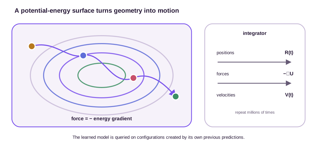
Numerical integration replaces the differential equation by finite updates. Velocity Verlet, for example, uses
\[\begin{aligned} \mathbf{r}_i^{n+1} &=\mathbf{r}_i^n +\Delta t\,\mathbf{v}_i^n +\frac{\Delta t^2}{2m_i}\mathbf{F}_i^n,\\ \mathbf{v}_i^{n+1} &=\mathbf{v}_i^n +\frac{\Delta t}{2m_i} \left(\mathbf{F}_i^n+\mathbf{F}_i^{n+1}\right). \end{aligned}\]The time step must resolve the fastest relevant motion. Making the force evaluation faster does not permit an arbitrarily larger \(\Delta t\): stiff bond vibrations and steep repulsive walls remain stiff. An unstable integrator and an unstable force field can look similar, so the time step must be converged independently.
One harmonic mode separates surface and integration error
A single harmonic coordinate makes the feedback loop executable. Set mass \(m=1\) and potential
\[U(x)=\frac12kx^2, \qquad F(x)=-kx, \qquad \omega=\sqrt{k/m}.\]Choose \(k=4\), so the exact angular frequency is \(\omega=2\) and the period is \(\pi\). Start at \(x_0=1\) and \(v_0=0\). With step \(h=0.4\), the initial force is \(F_0=-4\). A complete Velocity-Verlet step gives
\[x_1 =1+0.4(0)+\frac{0.4^2}{2}(-4) =0.68,\]then \(F_1=-4(0.68)=-2.72\) and
\[v_1 =0+\frac{0.4}{2}(-4-2.72) =-1.344.\]The exact solution at the same time is \(x(0.4)=\cos(0.8)\approx0.6967\) and \(v(0.4)=-2\sin(0.8)\approx-1.4347\). One finite step already creates phase and amplitude error even though the force is exact. The initial energy is 2; the numerical state has
\[H_1=\frac12(1.344)^2+2(0.68)^2 =1.8280.\]Velocity Verlet is symplectic: its energy error remains bounded and oscillatory in the stable regime rather than drifting monotonically as this one-step deficit might suggest. “Energy not exact after one step” and “unstable simulation” are different diagnoses.
For the harmonic system, the full update is linear:
\[\begin{bmatrix}x_{n+1}\\v_{n+1}\end{bmatrix} = \begin{bmatrix} 1-\frac12h^2\omega^2 & h\\ -h\omega^2\left(1-\frac14h^2\omega^2\right) &1-\frac12h^2\omega^2 \end{bmatrix} \begin{bmatrix}x_n\\v_n\end{bmatrix}.\]The matrix has determinant one and trace \(2-h^2\omega^2\). Its eigenvalues lie on the unit circle when
\[\lvert2-h^2\omega^2\rvert\leq2, \qquad\text{or equivalently}\qquad h\omega\leq2.\]Bounded generic trajectories require the strict inequality \(h\omega<2\). At the boundary \(h\omega=2\), the repeated eigenvalue is \(-1\) and the update matrix is generally not diagonalizable, allowing linear growth for generic initial velocities. This subtle boundary case is one reason production steps stay comfortably below a nominal stability limit.
For \(h=0.4\), \(h\omega=0.8\) and the motion is stable. Its numerical phase per step satisfies \(\cos\theta=1-(h\omega)^2/2=0.68\), giving \(\theta\approx0.823\) rather than the exact \(0.8\). At \(h=0.9\) the method remains formally stable because \(h\omega=1.8\), but \(\theta=\arccos(-0.62)\approx2.24\) instead of 1.8. The 24% phase error makes time correlations unreliable. At \(h=1.1\), \(h\omega=2.2\) and one eigenvalue leaves the unit circle, so amplitudes grow exponentially even on the exact potential.
This calculation supplies a differential diagnosis. If reducing \(h\) from 1.1 to 0.4 removes the blow-up while keeping the potential fixed, the integrator caused it. If the trajectory remains bounded but oscillates at the wrong limiting frequency as \(h\to0\), the surface caused it. If both frequency and integration converge but a finite trajectory gives a noisy mean, the remaining problem is sampling.
In a molecule, the relevant \(\omega\) is the largest eigenfrequency of the mass-weighted Hessian, not an average vibrational frequency. A single stiff X–H stretch can set the stable time step for thousands of slower collective coordinates. Constraints can remove selected fast modes, but then constraint tolerance and algorithmic error join the numerical budget.
In ideal isolated dynamics, the Hamiltonian
\[H(\mathbf{R},\mathbf{V}) =\sum_i\frac{m_i}{2}\lVert\mathbf{v}_i\rVert^2 +U(\mathbf{R})\]is conserved. This defines the microcanonical, or NVE, ensemble after equilibration. A thermostat instead exchanges energy with an idealized environment. Underdamped Langevin dynamics takes the form
\[d\mathbf{r}_i=\mathbf{v}_i\,dt,\] \[m_i\,d\mathbf{v}_i =\mathbf{F}_i\,dt -m_i\gamma\mathbf{v}_i\,dt +\sqrt{2m_i\gamma k_{\mathrm B}T}\,d\mathbf{W}_i.\]Friction removes kinetic energy and Brownian forcing restores it. Their fluctuation–dissipation relation makes the canonical density proportional to \(\exp[-H/(k_{\mathrm B}T)]\) stationary under suitable conditions. This is the NVT ensemble. A barostat adds volume or cell degrees of freedom to target pressure, producing an NPT ensemble. The Fokker–Planck post explains how the Langevin SDE induces this probability evolution.
The thermostat is not a repair mechanism for a bad potential. It controls ensemble sampling; it should not be expected to hide energy discontinuities, runaway forces, or missing physics.
A machine-learned force field approximates a reference surface
First-principles electronic-structure calculations provide accurate energies and forces but are too expensive for many large or long simulations. Classical force fields are much cheaper because they prescribe bonded, electrostatic, and dispersion terms, but their fixed functional forms can limit chemical accuracy and transferability. Machine-learned interatomic potentials aim at the middle: learn the reference potential with an evaluation cost closer to an empirical model.
The influential Behler–Parrinello construction writes the energy as a sum of atomic contributions (Behler & Parrinello, 2007):
\[U_\theta(\mathbf{Z},\mathbf{R}) =\sum_{i=1}^N \varepsilon_{\theta,i}.\]Here \(\mathbf{Z}\) contains chemical species. Local descriptors or a geometric neural network encode each environment, and shared parameters make the model size-extensive. Modern equivariant potentials improve data efficiency by letting vectors and higher-order geometric features transform consistently (Batzner et al., 2022). Their architectural details are the subject of the equivariant-potentials post.
For simulation, forces should usually be differentiated from the same scalar energy:
\[\mathbf{F}_{\theta,i} =-\nabla_{\mathbf{r}_i}U_\theta.\]This guarantees a conservative learned force field up to numerical differentiation. Translation invariance implies zero net internal force, rotation invariance implies the correct force transformation and zero net internal torque, and mixed derivatives obey the symmetries of an energy Hessian. A direct vector-force model may be accurate at sampled points while violating these integrability constraints between them.
Training commonly combines energy and force errors:
\[\mathcal{L}(\theta) =w_E\left(U_\theta-U^\star\right)^2 +\frac{w_F}{3N} \sum_{i=1}^N \left\lVert \mathbf{F}_{\theta,i}-\mathbf{F}_i^\star \right\rVert^2.\]Energy labels anchor relative basin depths; force labels constrain the local slope in \(3N\) coordinate directions. Stresses or virials are also important when cell response and pressure matter. The weights are not mere tuning constants: they determine which parts of the reference surface are reproduced most faithfully.
The reference method itself remains part of the model definition. An ML potential cannot systematically exceed the physics of its labels. Density-functional approximation, basis settings, dispersion treatment, spin state, charge state, and boundary conditions all propagate into the learned surface.
A stable learned oscillator can sample the wrong ensemble
Return to the harmonic reference \(U^\star(x)=2x^2\), but suppose the learned surface is
\[U_\theta(x)=\frac12\widehat{k}x^2, \qquad \widehat{k}=4.4.\]The force error is systematic: \(F_\theta-F^\star=-0.4x\). The learned frequency is
\[\widehat\omega=\sqrt{4.4}\approx2.098,\]which is 4.88% too high. Velocity Verlet with \(h=0.4\) remains safely inside its stability region because \(h\widehat\omega\approx0.839<2\). Smaller time steps converge to the dynamics of this learned oscillator, but they cannot recover the reference frequency of 2.
The equilibrium bias is equally explicit. At temperature \(k_{\mathrm B}T=1\), a harmonic canonical distribution has
\[p(x)\propto\exp\!\left(-\frac{kx^2}{2}\right), \qquad \langle x^2\rangle=\frac{1}{k}.\]The reference variance is \(1/4=0.25\). The learned variance is \(1/4.4\approx0.2273\), a 9.09% deficit. The simulation can remain bounded, conserve the learned Hamiltonian, and produce a sharply converged estimate of 0.2273. All three properties are compatible with the wrong scientific answer.
The same perturbation connects training loss to the surface. Under the reference canonical distribution, \(\mathbb E[x^2]=0.25\), so the force RMSE is
\[\sqrt{\mathbb E[(0.4x)^2]} =0.4\sqrt{0.25} =0.2.\]The energy error is \(U_\theta-U^\star=0.2x^2\). Its mean is 0.05, while its variation across \(x\) constrains curvature and relative weights. Force labels densely constrain local slopes, but a force-only fit is insensitive to independent energy constants on disconnected configuration components. Energy differences anchor basin offsets; forces determine local geometry. Their weights should reflect the intended observable and label units, not only make two numerical loss terms similar in magnitude.
Reference fidelity sits upstream of both terms. If a density-functional approximation yields curvature 4.4 while the physical target has curvature 4, an exact learner reproduces the 0.2273 variance of its reference. The quantum-chemistry post explains the electronic approximations that define this label surface. This chapter begins after that choice and asks what its learned surrogate does inside a simulation.
Training data should cover a distribution of environments, not frames from one movie
Consecutive frames of an ab initio trajectory are strongly correlated. Collecting more adjacent frames may increase dataset size without adding new local environments. Conversely, a rare compressed bond or transition-state geometry can be more valuable than thousands of equilibrium snapshots.
A useful dataset spans the conditions the production simulation will visit: phases, compositions, temperatures, pressures, strains, interfaces, defects, reaction coordinates, and high-energy repulsive configurations that act as guardrails. The split should respect this structure. Randomly splitting neighboring frames leaks almost identical geometries into train and test sets and produces an overly optimistic error estimate.
When the relevant configuration space is not known in advance, simulation and data generation can be coupled. A concurrent-learning loop trains several models, explores with the current potential, measures disagreement, labels selected configurations with the expensive reference method, and retrains. DP-GEN formalized this explore–label–train cycle for deep potentials (Zhang et al., 2020).
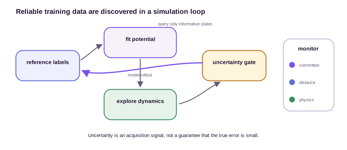
For an ensemble of \(M\) models, a simple force-disagreement score is
\[u(\mathbf{R}) =\max_i \sqrt{ \frac{1}{M} \sum_{m=1}^M \left\lVert \mathbf{F}^{(m)}_i -\overline{\mathbf{F}}_i \right\rVert^2 }.\]Large disagreement is evidence that the models are not constrained to the same answer. Small disagreement is weaker evidence: all members may share the same bias, representation limit, or missing physical term. Uncertainty is therefore useful for triage, not a certificate of correctness. It must be calibrated on genuinely shifted validation sets and supplemented by physical monitors such as minimum distances, maximum forces, energy drift, coordination changes, and known conservation laws.
Frame count is not sample count
Correlation reduces both the information in a training movie and the precision of a production estimate. Let \(A_n\) be an observable recorded every simulation step, with normalized lag correlation \(\rho_\ell\). A common definition of the integrated autocorrelation time in units of saved frames is
\[\tau_{\mathrm{int}} =1+2\sum_{\ell=1}^{\infty}\rho_\ell.\]For \(N\) stationary frames, the effective sample size is approximately
\[N_{\mathrm{eff}}\approx\frac{N}{\tau_{\mathrm{int}}}.\]Suppose \(\rho_\ell=0.9^\ell\). Then
\[\tau_{\mathrm{int}} =1+2\frac{0.9}{1-0.9} =19.\]A trajectory with 10,000 stored frames contains only about 526 effectively independent observations for that observable. Randomly placing adjacent frames into training and test sets hides the same factor: test configurations one step away from training are not independent evidence of deployment generalization. Thinning every 19th frame reduces storage correlation but does not create new basin visits; a trajectory trapped in one basin remains one-basin data however aggressively it is thinned.
Ensemble disagreement has a similarly precise limitation. At \(x=1\), three harmonic models with spring constants 4.2, 4.4, and 4.6 predict forces \(-4.2,-4.4,-4.6\). Their population standard deviation is about 0.163, so the state would plausibly be queried. But if all three training runs converge to the shared biased curvature 4.4, disagreement is exactly zero while their force differs from the reference by 0.4 and their canonical variance is wrong by 9.09%. Ensembles detect sensitivity to data, initialization, or model choice represented across their members. They cannot expose an error source shared by every member.
Active learning should therefore combine at least three signals. Disagreement identifies epistemically unstable regions. Geometric guardrails catch obviously unsafe states such as compressed bonds even when all models agree. Reference validation on shifted structures detects shared bias. The expensive label should be requested because it changes a decision boundary or expands physical coverage, not merely because a scalar uncertainty score is large.
Static error and rollout stability answer different questions
Suppose two potentials have the same force RMSE on a held-out set. One may still have a rough energy surface between test points, a discontinuous cutoff, or an unphysical low-energy pocket just outside the sampled domain. Molecular dynamics actively searches such defects because forces direct the trajectory toward whatever the model declares favorable.
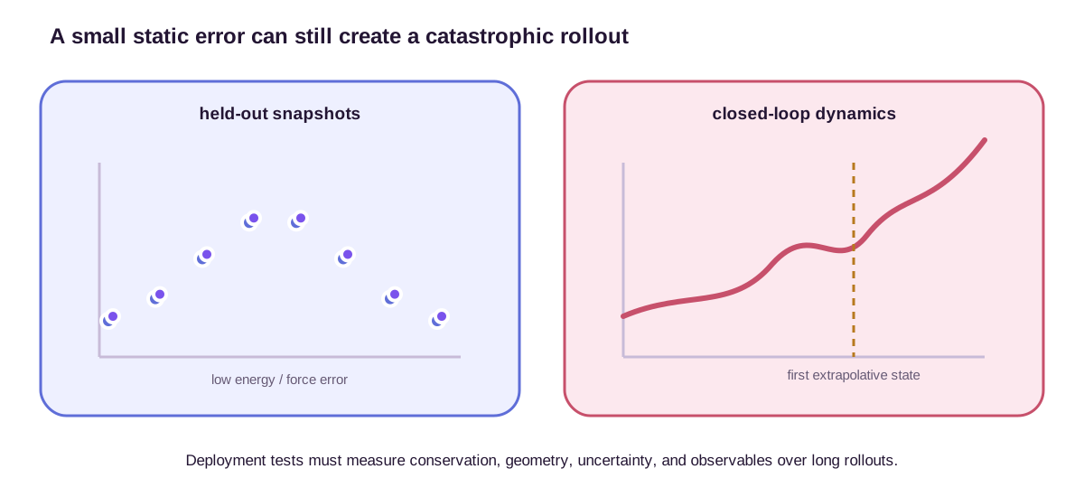
This creates several distinct failure modes:
- Integrator instability: \(\Delta t\) is too large for the fastest modeled mode.
- Surface roughness: energy is accurate but its derivatives change sharply, especially near a cutoff.
- Uncovered configuration: the trajectory enters chemistry or geometry absent from training.
- Spurious attraction: the model invents an artificial low-energy structure and the dynamics collapses into it.
- Systematic thermodynamic bias: the trajectory remains visually plausible but basin populations or pressures are wrong.
Fu et al. show that lower held-out errors do not automatically improve downstream physical predictions and propose energy conservation in molecular dynamics as an additional gate (Fu et al., 2025). Conservation is especially diagnostic in NVE simulation, where thermostatting cannot obscure the drift. It is necessary but not sufficient: a smooth conservative model can conserve the wrong Hamiltonian perfectly.
Rollout validation should therefore be adversarial. Start from multiple basins and temperatures; test longer than the training trajectories; perturb bonds and cell parameters; cross phase boundaries if they are in scope; and compare failure time as well as average error. Monitor the distribution of uncertainty over time, not only its mean. A rare peak often matters more than a low average.
Path divergence is not automatically distributional failure
Two chaotic molecular trajectories started from nearly identical states will separate exponentially even under the same exact potential. If their initial displacement is \(\delta_0\) and the largest Lyapunov exponent is \(\lambda>0\), the linear regime behaves roughly as
\[\delta(t)\approx\delta_0e^{\lambda t}.\]With \(\lambda=1\ \mathrm{ps}^{-1}\), an initial difference of \(10^{-6}\) grows to order one after about \(\log(10^6)\approx13.8\) ps. A learned and reference trajectory need not remain pointwise aligned for longer than this even when they sample nearly identical equilibrium distributions. Trajectory RMSD is therefore a short-time diagnostic, not a universal long-time accuracy metric.
The converse also fails. The biased harmonic model follows perfectly regular periodic paths and can remain close to the reference for several cycles, yet its limiting canonical variance is 9.09% low. Path plausibility does not establish correct stationary weights. For equilibrium claims, compare distributions or observables. For kinetic claims, compare time-correlation functions, transition rates, or transport coefficients under a dynamics protocol that preserves their meaning.
Step-size refinement separates another pair of causes. Run the same initial conditions and model with \(h,h/2,h/4\). If NVE energy drift or an observable changes systematically and converges as \(h\to0\), discretization is implicated. If the limit stabilizes at the wrong frequency or variance, the learned surface is implicated. If estimates wander without a trend and block uncertainty shrinks with trajectory length, estimator variance or insufficient mixing is implicated. Changing the thermostat may reduce a temperature-control symptom while leaving the wrong learned curvature untouched; it is not a matched intervention for surface error.
Local models need explicit answers for long-range physics
Most scalable ML potentials use a finite neighborhood radius. This makes evaluation approximately linear in atom count and matches the locality of many short-range interactions. It also creates two obligations.
First, energy and its required derivatives must vanish smoothly at the cutoff. If an edge disappears abruptly, the force changes discontinuously. Repeating that discontinuity over many neighbor-list crossings produces heating or energy drift.
Let one radial contribution be \(E(r)=\phi(r)c(r)\) for \(r<r_c\) and zero outside. The switching function \(c\) carries the cutoff. Its radial force inside is
\[F(r)=-\frac{dE}{dr} =-\phi'(r)c(r)-\phi(r)c'(r).\]Energy continuity for an arbitrary finite \(\phi(r_c)\) requires \(c(r_c)=0\). A force that also approaches zero continuously requires \(c'(r_c)=0\). If Hessians, vibrational frequencies, or smooth force derivatives matter, then \(c''(r_c)=0\) is the next obligation. A cosine cutoff
\[c(r)=\frac12\left[1+\cos\!\left(\frac{\pi r}{r_c}\right)\right]\]has zero value and slope at \(r_c\), but its second derivative jumps when joined to zero outside. A quintic switch over a normalized interval \(s\in[0,1]\),
\[c(s)=1-10s^3+15s^4-6s^5,\]has zero first and second derivatives at both ends. The appropriate smoothness is set by the downstream observable: stable forces require less than phonon spectra or higher-order response. Neighbor-list bookkeeping must include a skin region so pairs are not omitted between rebuilds even when the analytic cutoff is smooth.
Second, a local environment is not always sufficient. Electrostatics, polarization, dispersion, and charge transfer can couple distant regions. Two atoms may have identical neighbors inside the cutoff but belong to systems with different total charge or electric field. No amount of local training data can resolve information excluded from the representation.
This is an information-theoretic failure, not an optimization failure. Place a tagged neutral local cluster inside radius \(r_c\) and consider two otherwise identical systems with a distant charge \(+q\) at \(+R\) in one and \(-q\) at \(+R\) in the other, where \(R>r_c\). Every local descriptor of the tagged cluster is identical, yet the external electric fields have opposite directions and induce different forces or polarization energies. A strictly local deterministic model must return the same answer for both. More data cannot make a function distinguish inputs that its representation maps to the same value.
The remedy depends on the physics: add explicit electrostatics or dispersion, predict environment-dependent charges and solve a global charge-equilibration problem, use reciprocal-space components, or combine local and global message passing. Fourth-generation high-dimensional neural-network potentials demonstrate how nonlocal charge equilibration can complement local energy terms (Ko et al., 2021). The important decision is explicit: identify which interactions are delegated to learning and which are retained as structured physics.
Long-range adequacy should be tested at the observable level. A model can have excellent short-range force errors yet fail dielectric response, interfacial energetics, phonons, or diffusion because a weak missing interaction accumulates coherently across the system.
The simulation workflow defines what can be measured
A production trajectory is not obtained by placing atoms in a box and pressing run. A typical workflow minimizes severe overlaps, ramps temperature, equilibrates the target ensemble, and only then accumulates production statistics. Initialization is consequential because a metastable system may retain memory of its starting basin for far longer than the nominal equilibration period.
Observables fall into several classes. Structural quantities include radial distribution functions,
\[g(r) =\frac{1}{4\pi r^2\rho N} \left\langle \sum_{i\neq j}\delta(r-r_{ij}) \right\rangle,\]coordination numbers, angular distributions, and conformational populations. Thermodynamic quantities include mean energy, pressure, heat capacity, phase stability, and free-energy differences. A free-energy difference between regions \(A\) and \(B\) can be written as
\[\Delta F_{A\to B} =-k_{\mathrm B}T \log\frac{P(B)}{P(A)},\]provided the simulation samples both regions with the correct equilibrium weights. Dynamic quantities include relaxation times and transport coefficients. For example, the Einstein relation gives the self-diffusion coefficient in three dimensions:
\[D =\lim_{t\to\infty} \frac{1}{6t} \left\langle \lVert\mathbf{r}_i(t)-\mathbf{r}_i(0)\rVert^2 \right\rangle.\]Basin counts need correlated-sample uncertainty
Suppose a production trajectory assigns 8,000 frames to basin \(A\) and 2,000 to basin \(B\). At face value,
\[\frac{P(B)}{P(A)}=\frac{2000}{8000}=0.25, \qquad \Delta F_{A\to B}=k_{\mathrm B}T\log4 \approx1.386\,k_{\mathrm B}T.\]Treating 10,000 correlated frames as 10,000 Bernoulli trials would understate uncertainty. Divide the trajectory into blocks longer than the basin-indicator autocorrelation time. If four effectively independent blocks have \(B\) fractions 0.15, 0.20, 0.25, and 0.20, their block free-energy estimates are approximately 1.735, 1.386, 1.099, and 1.386 in units of \(k_{\mathrm B}T\). Their mean is 1.402 and their standard error is about 0.130. The full-count estimate lies inside that uncertainty, but the block variation reveals how little information four transition-scale blocks contain.
Block averaging addresses estimator variance conditional on the sampled process. It does not correct a biased stationary distribution. If the learned curvature, basin offset, thermostat, or enhanced-sampling reweighting is wrong, longer simulation converges more confidently to the wrong free energy. Multiple starts and round trips between basins test mixing; comparisons against reference free energies test the surface and ensemble.
A diffusion estimate makes a kinetic claim
Suppose the long-lag mean-squared displacement is 6 square angstroms at 10 ps. The three-dimensional Einstein estimate is
\[D\approx\frac{6\ \text{Å}^2}{6(10\ \mathrm{ps})} =0.10\ \text{Å}^2/\mathrm{ps} =1.0\times10^{-9}\ \mathrm{m}^2/\mathrm{s}.\]This number is meaningful only if the mean-squared-displacement curve has entered a linear diffusive regime. At short lags, ballistic motion gives quadratic growth. In a finite periodic cell, hydrodynamic finite-size effects can shift the slope. Multiple time origins reduce variance, but overlapping origins are correlated and require block or replicate uncertainty.
These formulas expose two different validation requirements. Equilibrium averages require correct stationary weights and adequate mixing. Kinetic quantities additionally require faithful time correlations. An aggressive thermostat, coarse-graining, or biased enhanced-sampling force may preserve or recover equilibrium statistics after reweighting while distorting real dynamics. A strong Langevin friction or metadynamics bias can accelerate decorrelation while making the raw Einstein slope nonphysical. One trajectory can support an equilibrium claim and fail to support a kinetic one.
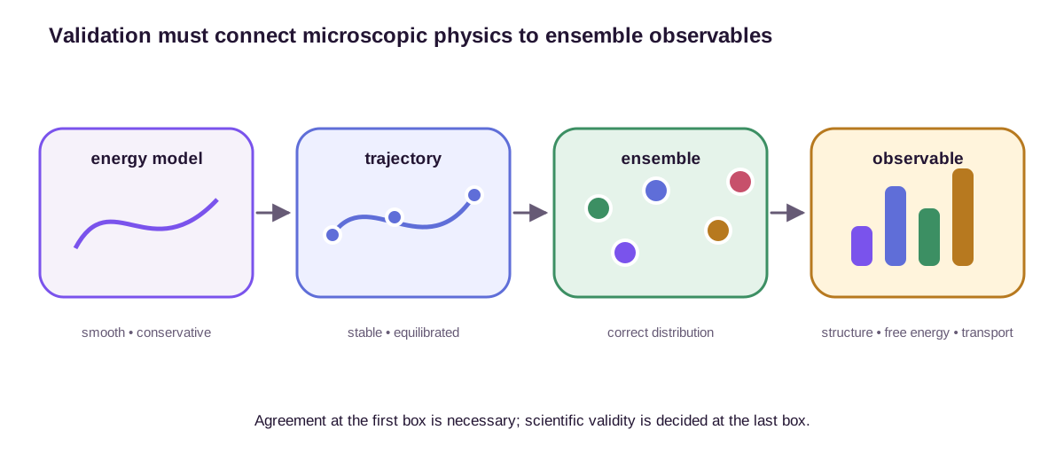
Rare events make the distinction sharper. If a barrier crossing is much slower than the accessible trajectory, an unbiased simulation may be stable but statistically useless. Replica exchange, metadynamics, umbrella sampling, and learned bias potentials accelerate exploration, but their bias and reweighting rules become part of the estimator. Faster sampling does not relax the need for an accurate underlying potential in the visited regions.
Validation should follow the intended claim
A simulation-ready validation report should separate four layers.
At the reference layer, verify energy, force, virial, and relative-energy errors on splits organized by trajectory, composition, phase, and thermodynamic condition. At the dynamical layer, measure NVE drift, temperature and pressure control, constraint violations, neighbor-list smoothness, and catastrophic-failure time across seeds. At the distribution layer, compare structural distributions and basin populations, with block averaging and effective sample sizes to account for autocorrelation. At the observable layer, compare the actual claimed quantities—free energies, diffusion, elastic constants, phonons, reaction rates, or phase boundaries—with reference calculations or experiment, including statistical and model uncertainty.
This hierarchy prevents a common category error. A low force RMSE supports the claim that local derivatives interpolate well on a particular test distribution. It does not by itself support a melting temperature, binding free energy, or diffusion coefficient. Those claims require the entire trajectory-to-estimator pipeline.
Vary one axis at a time
A convergence study is informative only if its intervention matches the suspected error. The following matrix separates the main budgets.
| Error source | Controlled variation | Diagnostic that should respond | What convergence cannot establish |
|---|---|---|---|
| Reference physics | Functional, basis, dispersion, spin, cell size | Recomputed energy differences, forces, barriers | Accuracy beyond the compared reference family |
| Learned surface | Dataset coverage, model capacity, energy/force weights, ensemble | Shifted-set errors, curvature, disagreement, adversarial rollout | Correct time integration or adequate sampling |
| Discretization | \(h,h/2,h/4\) at fixed surface and protocol | NVE drift, phase, constraint error, observable extrapolation in \(h\) | Correctness of the limiting learned Hamiltonian |
| Transient and mixing | Burn-in, independent starts, trajectory length, enhanced sampling | Basin round trips, stationarity, autocorrelation time | Correct stationary weights if the potential or reweighting is biased |
| Estimator variance | Block size, independent replicas, number of particles and time origins | Standard error and confidence-interval stability | Removal of systematic model, ensemble, or finite-size bias |
| Finite-size and boundary effects | Box length, particle count, reciprocal-space settings | Size scaling of pressure, diffusion, dielectric response | Transfer to another composition or thermodynamic state |
The harmonic example runs through the middle four rows. Decreasing \(h\) below 0.4 makes the numerical frequency converge. With the true surface it converges to 2; with \(\widehat k=4.4\) it converges to 2.098. Increasing the thermostatted trajectory length reduces uncertainty in \(\langle x^2\rangle\), but the two surfaces converge to 0.25 and 0.2273 respectively. An ensemble whose members all use \(\widehat k=4.4\) reports zero disagreement. No one-axis success crosses into another row.
For a molecular production claim, the same logic suggests a staged protocol. First fix the reference and validate relative energies and derivatives on independent physical groups. Then freeze the model and reduce the integration step until the claimed observable changes less than its statistical tolerance. Next freeze model and step, extend or replicate trajectories until basin indicators and observables have stable block errors. Finally vary system size or boundary treatment if the observable is nonlocal. At each stage, report the quantity held fixed; otherwise simultaneous changes to model, thermostat, and step size make an improvement impossible to attribute.
The final comparison must target the claim. A force field intended for equilibrium liquid structure needs radial distributions, densities, and composition-aware free energies. A potential intended for vibrational spectra needs smooth Hessians and accurate phase correlations. A reactive potential needs barrier regions, products, and guardrails against spurious channels. A transport potential needs the physical dynamical protocol, long-time linear regimes, and finite-size checks. The word “stable” contributes only one gate: the trajectory did not catastrophically fail under the tested conditions.
Machine-learned force fields are powerful precisely because they turn costly electronic-structure information into long trajectories. The leverage is enormous, and so is the opportunity for errors to compound. The right standard is therefore not whether a network is accurate once. It is whether the learned surface, numerical dynamics, sampled ensemble, and final observable remain mutually consistent for the full simulation the scientist intends to trust.
References
- Behler, J., & Parrinello, M. (2007). Generalized neural-network representation of high-dimensional potential-energy surfaces. Physical Review Letters, 98, 146401. ↩
- Batzner, S., Musaelian, A., Sun, L., Geiger, M., Mailoa, J. P., Kornbluth, M., Molinari, N., Smidt, T. E., & Kozinsky, B. (2022). E(3)-equivariant graph neural networks for data-efficient and accurate interatomic potentials. Nature Communications, 13, 2453. ↩
- Zhang, Y., Wang, H., Chen, W., Zeng, J., Zhang, L., Wang, H., & E, W. (2020). DP-GEN: A concurrent learning platform for the generation of reliable deep learning based potential energy models. Computer Physics Communications, 253, 107206. ↩
- Fu, X., Wood, B. M., Barroso-Luque, L., Levine, D. S., Gao, M., Dzamba, M., & Zitnick, C. L. (2025). Learning smooth and expressive interatomic potentials for physical property prediction. Proceedings of the 42nd International Conference on Machine Learning, 17875–17893. ↩
- Ko, T. W., Finkler, J. A., Goedecker, S., & Behler, J. (2021). A fourth-generation high-dimensional neural network potential with accurate electrostatics including non-local charge transfer. Nature Communications, 12, 398. ↩
Figure provenance. All four molsim_ diagrams are original SVG illustrations generated by scripts/generate_molsim_figures.py. They synthesize standard simulation identities and the validation principles discussed in the cited primary literature; no third-party artwork is reproduced.