On this page
Note: This post is based on material I previously studied with Minkyu Kim. It presents the Fokker-Planck equation in three layers: physical intuition, a heuristic derivation via discretization (following Lai et al., 2025), and a rigorous derivation via Itô calculus. The first two layers use only multivariate calculus; the third introduces stochastic calculus for readers who want the full proof.
Introduction
Diffusion models, including DDPMs (Ho et al., 2020), score-based models (Song et al., 2021), and ODE counterparts such as flow matching (Lipman et al., 2023), are built on stochastic differential equations (SDEs) and their density dynamics. An SDE gradually corrupts data into noise; a learned reverse process turns noise back into data. The Fokker-Planck equation connects these two views: given an SDE for individual sample paths, it tells us how the probability density \(p_t(\mathbf{x})\) evolves over time. It is the starting point for deriving probability-flow ODEs, reverse-time SDEs, and score-matching objectives.
Most diffusion-model tutorials state the Fokker-Planck equation without proof and move on. A rigorous derivation requires Itô calculus, which is not part of the standard ML curriculum. This post takes three passes at the equation: first the picture, then a multivariate-calculus derivation following Lai et al., 2025, then the Itô proof.
The Fokker-Planck Equation
Consider a stochastic process \(\{\mathbf{x}(t)\}_{t \in [0,T]}\) in \(\mathbb{R}^D\) governed by an SDE:
SDE. The process evolves according to
\[d\mathbf{x}(t) = \mathbf{f}(\mathbf{x}(t), t)\,dt + g(t)\,d\mathbf{w}(t)\]where \(\mathbf{f}: \mathbb{R}^D \times [0,T] \to \mathbb{R}^D\) is the drift (a deterministic force pushing the particle), \(g: [0,T] \to \mathbb{R}\) is the diffusion coefficient (the intensity of random noise), and \(\mathbf{w}(t)\) is a standard \(D\)-dimensional Wiener process (Brownian motion). The initial condition is \(\mathbf{x}(0) \sim p_0\).
The SDE describes one particle path: at each instant, the particle drifts by \(\mathbf{f}(\mathbf{x},t)\,dt\) and receives a random kick of magnitude \(g(t)\,d\mathbf{w}\). Our goal is the PDE for the marginal density \(p_t(\mathbf{x})\), the probability of finding the particle at position \(\mathbf{x}\) at time \(t\). That PDE is the Fokker-Planck equation:
Fokker-Planck Equation. The density \(p_t(\mathbf{x})\) evolves according to
\[\displaystyle\frac{\partial p_t(\mathbf{x})}{\partial t} = \underbrace{-\nabla_{\mathbf{x}} \cdot \bigl[\mathbf{f}(\mathbf{x},t)\,p_t(\mathbf{x})\bigr]}_{\text{advection by drift}} + \underbrace{\frac{g^2(t)}{2}\,\Delta_{\mathbf{x}}\,p_t(\mathbf{x})}_{\text{spreading by diffusion}}\]where \(\nabla_{\mathbf{x}} \cdot [\,\cdot\,]\) is the divergence operator and \(\Delta_{\mathbf{x}} = \sum_{i=1}^{D} \frac{\partial^2}{\partial x_i^2}\) is the Laplacian.
Before deriving the equation, we build intuition for each term. The derivation also uses the transition kernel, the Gaussian conditional distribution obtained by discretizing the SDE.
For a small time step \(\Delta t\), the Euler-Maruyama approximation gives
\[\mathbf{x}_{t+\Delta t} = \mathbf{x}_t + \mathbf{f}(\mathbf{x}_t, t)\,\Delta t + g(t)\sqrt{\Delta t}\;\boldsymbol{\epsilon}\]with \(\boldsymbol{\epsilon} \sim \mathcal{N}(\mathbf{0}, \mathbf{I})\), so:
Euler–Maruyama transition kernel. The discretized step has a Gaussian conditional distribution; the exact SDE transition need not be Gaussian:
\[p(\mathbf{x}_{t+\Delta t} \mid \mathbf{x}_t) = \mathcal{N}\!\left(\mathbf{x}_{t+\Delta t};\; \mathbf{x}_t + \mathbf{f}(\mathbf{x}_t, t)\,\Delta t,\; g^2(t)\,\Delta t\;\mathbf{I}\right)\]The mean is the current position shifted by the drift, and the variance is \(g^2(t)\,\Delta t\) in each coordinate.
Advection by Drift
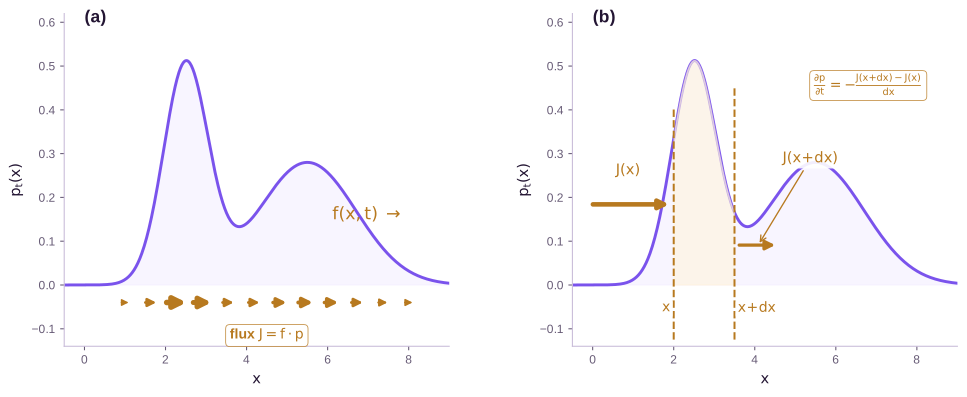
The quantity \(\mathbf{f}\,p_t\) is a probability flux: density times velocity. The negative divergence \(-\nabla \cdot (\mathbf{f}\,p_t)\) measures net inflow. Where flux converges, density accumulates; where it diverges, density depletes. In one dimension, this becomes the finite-difference statement \(\partial_t p = -(J(x{+}\Delta x) - J(x))/\Delta x\): density in a slab changes by the net flux through its boundaries. With no noise (\(g = 0\)), the equation reduces to the continuity equation from fluid dynamics.
Spreading by Diffusion
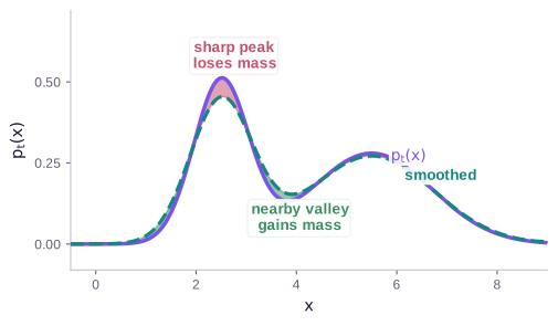
At each instant, the SDE’s noise kicks every particle by a symmetric random displacement \(g\,d\mathbf{w}\). The aggregate effect is Gaussian blurring: peaks erode and valleys fill.
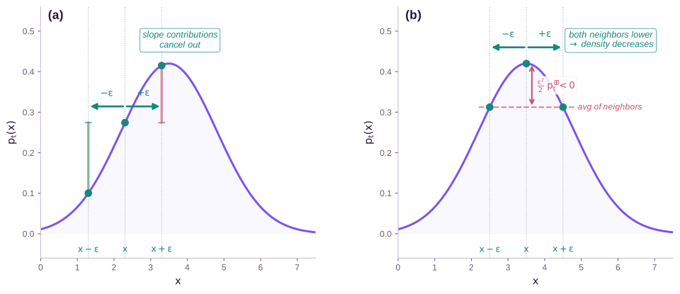
Why does blurring produce a second derivative? In a small time step \(\Delta t\), the noise moves each particle from \(y\) to \(y + \epsilon\), where \(\epsilon \sim \mathcal{N}(0,\, g^2\,\Delta t)\). A particle arrives at \(x\) only if it started at \(y\) and received kick \(\epsilon = x - y\). Summing over starting positions, weighted by the density \(p_t(y)\) and the probability of the required kick:
\[p_{t+\Delta t}(x) = \int p_t(y)\;\mathcal{N}\!\left(x - y;\;0,\,g^2\,\Delta t\right)dy = \mathbb{E}_\epsilon\!\left[p_t(x - \epsilon)\right]\]where the second equality substitutes \(\epsilon = x - y\). Taylor-expanding \(p_t(x - \epsilon)\) around \(x\):
\[p_t(x - \epsilon) \approx p_t(x) \;-\; \epsilon\,p_t'(x) \;+\; \frac{\epsilon^2}{2}\,p_t''(x)\]Now take the expectation term by term:
-
The linear term \(-\epsilon\,p_t'(x)\) vanishes. A kick \(+\epsilon\) to the right is exactly as likely as \(-\epsilon\) to the left, so \(\mathbb{E}[\epsilon] = 0\) and the slope contributions cancel.
-
The quadratic term \(\frac{\epsilon^2}{2}\,p_t''(x)\) survives. Whether the particle goes left or right, \(\epsilon^2\) is positive — the direction cancels but the magnitude does not. This term detects curvature: whether neighbors on both sides have higher density than \(x\) (\(p_t'' > 0\), valley) or lower (\(p_t'' < 0\), peak).
To first order in time, the curvature term remains: \(p_{t+\Delta t}(x) = p_t(x) + \frac{g^2\,\Delta t}{2}\,p_t''(x) + o(\Delta t)\). Dividing by \(\Delta t\) and taking the limit gives the diffusion PDE in one dimension:
\[\displaystyle\frac{\partial p_t}{\partial t} = \frac{g^2}{2}\,\frac{\partial^2 p_t}{\partial x^2}\]In \(D\) dimensions, the noise components \(dw_1, \ldots, dw_D\) are independent, so the same argument applies along each coordinate, giving \(\frac{g^2}{2}\,\Delta_{\mathbf{x}}\,p_t\).
Deriving the Fokker-Planck Equation
This section gives a heuristic derivation based on Euler-Maruyama discretization. It produces the correct equation and shows where each term comes from, but it hides regularity conditions: we exchange limits, integrals, and Taylor expansions without justifying when those operations are valid. The next section gives the rigorous derivation via Itô calculus.
The derivation proceeds from the Gaussian transition kernel in three steps.
Step 1: Chapman-Kolmogorov
For the Euler–Maruyama approximation, the next marginal density is obtained by integrating its transition kernel against the current density. We use \(p_t\) for the discretized marginals in this heuristic section and then pass to the continuous-time limit:
Chapman-Kolmogorov equation. The marginal density at time \(t + \Delta t\) is
\[p_{t+\Delta t}(\mathbf{x}) = \int \mathcal{N}\!\left(\mathbf{x};\; \mathbf{y} + \mathbf{f}(\mathbf{y},t)\,\Delta t,\; g^2(t)\,\Delta t\;\mathbf{I}\right) p_t(\mathbf{y})\,d\mathbf{y}\]This is marginalization: sum over all previous positions \(\mathbf{y}\), weighted by their density \(p_t(\mathbf{y})\) and the transition probability \(\mathbf{y} \to \mathbf{x}\). The Markov property justifies using only the one-step kernel.
Step 2: Change of Variables
The Gaussian kernel is centered at \(\mathbf{y} + \mathbf{f}(\mathbf{y},t)\,\Delta t\), which depends on \(\mathbf{y}\). To simplify the integral, introduce a new variable that absorbs the drift:
\[\mathbf{u} := \mathbf{y} + \mathbf{f}(\mathbf{y},t)\,\Delta t\]Now the Gaussian is centered at \(\mathbf{u}\): \(\mathcal{N}(\mathbf{x};\;\mathbf{u},\;g^2(t)\,\Delta t\;\mathbf{I})\). For small \(\Delta t\), the map \(\mathbf{y} \mapsto \mathbf{u}\) is invertible. The inverse follows from substituting back into the definition of \(\mathbf{u}\) and dropping \(\mathcal{O}(\Delta t^2)\) cross-terms:
\[\mathbf{y} = \mathbf{u} - \mathbf{f}(\mathbf{u},t)\,\Delta t + \mathcal{O}(\Delta t^2)\]The Jacobian determinant uses the identity \(\det(\mathbf{I} - \mathbf{A}\,\Delta t) = 1 - \text{tr}(\mathbf{A})\,\Delta t + \mathcal{O}(\Delta t^2)\):
\[\left\lvert\det \frac{\partial \mathbf{y}}{\partial \mathbf{u}}\right\rvert = 1 - (\nabla_{\mathbf{u}} \cdot \mathbf{f})(\mathbf{u},t)\,\Delta t + \mathcal{O}(\Delta t^2)\]Substituting into the Chapman-Kolmogorov integral and Taylor-expanding \(p_t(\mathbf{y})\) around \(\mathbf{u}\):
\[p_t(\mathbf{y}) = p_t(\mathbf{u}) - \Delta t\;\mathbf{f}(\mathbf{u},t) \cdot \nabla_{\mathbf{u}} p_t(\mathbf{u}) + \mathcal{O}(\Delta t^2)\]Combining this with the Jacobian determinant produces two \(\Delta t\) corrections with distinct origins: one from the Taylor expansion of \(p_t\), because density varies across space, and one from the Jacobian, because the change of variables distorts volume elements:
\[\begin{aligned} p_{t+\Delta t}(\mathbf{x}) = \int \mathcal{N}\!\left(\mathbf{x};\;\mathbf{u},\;g^2(t)\,\Delta t\;\mathbf{I}\right) \Big[&\, p_t(\mathbf{u}) - \Delta t\;\mathbf{f}(\mathbf{u},t) \cdot \nabla_{\mathbf{u}} p_t(\mathbf{u}) \\ &- \Delta t\;(\nabla_{\mathbf{u}} \cdot \mathbf{f})(\mathbf{u},t)\;p_t(\mathbf{u})\Big] d\mathbf{u} + \mathcal{O}(\Delta t^2) \end{aligned}\]Step 3: Taylor-Gaussian Smoothing
Each term in the bracket is now convolved against a Gaussian \(\mathcal{N}(\mathbf{x};\;\mathbf{u},\;\sigma^2\mathbf{I})\) with \(\sigma^2 = g^2(t)\,\Delta t\). The Taylor expansion from the intuition section now applies in \(D\) dimensions.
Taylor-Gaussian smoothing. For any smooth function \(\phi: \mathbb{R}^D \to \mathbb{R}\) and \(\mathbf{z} \sim \mathcal{N}(\mathbf{0}, \mathbf{I})\):
\[\int \mathcal{N}(\mathbf{x};\;\mathbf{u},\;\sigma^2\mathbf{I})\;\phi(\mathbf{u})\,d\mathbf{u} = \mathbb{E}\!\left[\phi(\mathbf{x} + \sigma\mathbf{z})\right] = \phi(\mathbf{x}) + \frac{\sigma^2}{2}\,\Delta_{\mathbf{x}}\phi(\mathbf{x}) + \mathcal{O}(\sigma^4)\]Gaussian convolution equals the original function plus a Laplacian correction. The first-order term vanishes by symmetry (\(\mathbb{E}[\mathbf{z}] = \mathbf{0}\)); the second-order term survives because \(\mathbb{E}[z_i z_j] = \delta_{ij}\).
This follows from Taylor-expanding \(\phi(\mathbf{x} + \sigma\mathbf{z})\) to second order:
\[\phi(\mathbf{x} + \sigma\mathbf{z}) = \phi(\mathbf{x}) + \sigma\,\nabla_{\mathbf{x}}\phi(\mathbf{x}) \cdot \mathbf{z} + \frac{\sigma^2}{2}\,\mathbf{z}^\top \nabla_{\mathbf{x}}^2 \phi(\mathbf{x})\,\mathbf{z} + \mathcal{O}(\sigma^3)\]and taking expectations. The components of \(\mathbf{z}\) are independent standard normals, so \(\mathbb{E}[\mathbf{z}^\top \mathbf{A}\,\mathbf{z}] = \text{tr}(\mathbf{A})\). The trace of the Hessian is the Laplacian.
Now apply this identity to each term in the bracket. Since \(\sigma^2 = g^2(t)\,\Delta t\), the Gaussian smoothing of the leading term \(p_t(\mathbf{u})\) contributes a Laplacian at order \(\Delta t\):
\[\int \mathcal{N}(\mathbf{x};\;\mathbf{u},\;\sigma^2\mathbf{I})\;p_t(\mathbf{u})\,d\mathbf{u} = p_t(\mathbf{x}) + \frac{g^2(t)\,\Delta t}{2}\,\Delta_{\mathbf{x}}\,p_t(\mathbf{x}) + \mathcal{O}(\Delta t^2)\]For the two terms already at order \(\Delta t\), namely the drift-gradient and divergence terms, Gaussian smoothing leaves them unchanged at leading order; the \(\sigma^2\) correction would only produce \(\mathcal{O}(\Delta t^2)\) terms. Collecting everything:
\[\begin{aligned} p_{t+\Delta t}(\mathbf{x}) - p_t(\mathbf{x}) = \;&{-}\Delta t\;\mathbf{f}(\mathbf{x},t) \cdot \nabla_{\mathbf{x}} p_t(\mathbf{x}) - \Delta t\;(\nabla_{\mathbf{x}} \cdot \mathbf{f})(\mathbf{x},t)\;p_t(\mathbf{x}) \\ &+ \frac{g^2(t)}{2}\,\Delta t\;\Delta_{\mathbf{x}}\,p_t(\mathbf{x}) + \mathcal{O}(\Delta t^2) \end{aligned}\]The first two terms combine via the product rule: \(\mathbf{f} \cdot \nabla p + (\nabla \cdot \mathbf{f})\,p = \nabla \cdot (\mathbf{f}\,p)\). Dividing both sides by \(\Delta t\) and taking \(\Delta t \to 0\):
\[\frac{\partial p_t(\mathbf{x})}{\partial t} = -\nabla_{\mathbf{x}} \cdot \bigl[\mathbf{f}(\mathbf{x},t)\,p_t(\mathbf{x})\bigr] + \frac{g^2(t)}{2}\,\Delta_{\mathbf{x}}\,p_t(\mathbf{x})\]Rigorous Derivation via Itô Calculus
The heuristic derivation discretized the SDE, Taylor-expanded, and took limits. It produced the right answer, but without controlling error terms or justifying the interchange of limits and integrals. This section gives a weak-form derivation using Itô calculus. Assume the SDE is well posed, its coefficients make the integrals below integrable, and use smooth, compactly supported test functions. A classical density equation requires additional regularity; the integrated weak identity does not.
What Is Itô Calculus?
Ordinary calculus assumes smooth paths: differentiation and the chain rule require well-defined derivatives. Brownian motion \(\mathbf{w}(t)\) violates this assumption; its sample paths are continuous but nowhere differentiable. Writing \(d\mathbf{w}/dt\) is meaningless, so expressions such as \(d\mathbf{x} = \mathbf{f}\,dt + g\,d\mathbf{w}\) cannot be interpreted through classical calculus.
Itô calculus resolves this by redefining integration rather than differentiation:
Itô integral. The stochastic integral is defined as the limit
\[\displaystyle\int_0^T H(t)\,d\mathbf{w}(t) = \lim_{n \to \infty} \sum_{k=0}^{n-1} H(t_k)\bigl[\mathbf{w}(t_{k+1}) - \mathbf{w}(t_k)\bigr]\]The integrand \(H(t_k)\) is evaluated at the left endpoint of each subinterval, so it depends only on information available at time \(t_k\), before the increment \(\mathbf{w}(t_{k+1}) - \mathbf{w}(t_k)\) is realized.
The left-endpoint choice has two consequences that drive the derivation:
-
A square-integrable Itô integral is a martingale. For an adapted integrand with finite expected time-integrated squared norm, its expectation is zero: \(\mathbb{E}\!\left[\int_0^T H(t)\,d\mathbf{w}(t)\right] = 0\). Each increment \(\mathbf{w}(t_{k+1}) - \mathbf{w}(t_k)\) is independent of \(H(t_k)\) and has zero mean. In the Fokker-Planck derivation below, this property makes the stochastic integral disappear after taking expectations.
-
Quadratic variation is non-trivial. For smooth paths, \((dx)^2\) is negligible compared to \(dx\). For Brownian motion, \((d\mathbf{w})^2 = dt\): increments are order \(\sqrt{dt}\), so their squares accumulate at order \(dt\). Second-order Taylor terms therefore survive and produce the Itô correction in the chain rule.
These two facts — martingale property and non-vanishing quadratic variation — are the only tools we need. The following example shows both in action.
Example: computing \(\int_0^T W_t\,dW_t\). Write \(W_t = w(t)\) for a one-dimensional Brownian motion. Consider the simplest non-trivial Itô integral. (The multi-dimensional case follows coordinate-by-coordinate.)
Write the Itô sum and use the algebraic identity \(a(b-a) = \frac{1}{2}(b^2 - a^2) - \frac{1}{2}(b-a)^2\):
\[\sum_k W_{t_k}(W_{t_{k+1}} - W_{t_k}) = \frac{1}{2}\sum_k \bigl(W_{t_{k+1}}^2 - W_{t_k}^2\bigr) - \frac{1}{2}\sum_k (W_{t_{k+1}} - W_{t_k})^2\]The first sum telescopes to \(\frac{1}{2}W_T^2 - \frac{1}{2}W_0^2\). The second sum is the quadratic variation: each squared increment \((W_{t_{k+1}} - W_{t_k})^2\) has mean \(t_{k+1} - t_k\), and the variance of the full sum shrinks to zero as the partition refines. The sum converges to \(\frac{1}{2}T\), giving:
\[\int_0^T W_t\,dW_t = \frac{1}{2}W_T^2 - \frac{1}{2}W_0^2 - \frac{1}{2}T\]Had we instead evaluated at the right endpoint \(W_{t_{k+1}}\) (the backward Itô convention), the identity \(b(b-a) = \frac{1}{2}(b^2 - a^2) + \frac{1}{2}(b-a)^2\) gives \(\frac{1}{2}W_T^2 - \frac{1}{2}W_0^2 + \frac{1}{2}T\). The two answers differ by \(T\) — the full quadratic variation of Brownian motion over \([0,T]\). For smooth paths this difference vanishes and the evaluation point is irrelevant; for Brownian paths it is not.
Rearranging the Itô result reveals a stochastic chain rule:
\[d\!\left[\tfrac{1}{2}W_t^2\right] = W_t\,dW_t + \tfrac{1}{2}\,dt\]In ordinary calculus, \(d[\frac{1}{2}x^2] = x\,dx\). The extra \(\frac{1}{2}\,dt\) is the Itô correction — a direct consequence of \((dW_t)^2 = dt\).
Itô’s Lemma
The example above showed that the ordinary chain rule \(d[\frac{1}{2}x^2] = x\,dx\) gains an extra \(\frac{1}{2}\,dt\) for stochastic processes. Itô’s lemma generalizes this correction to arbitrary smooth functions.
Itô’s lemma. For the SDE \(d\mathbf{x} = \mathbf{f}\,dt + g\,d\mathbf{w}\) and a smooth function \(\varphi(\mathbf{x}, t)\):
\[d\varphi = \left(\frac{\partial \varphi}{\partial t} + \mathbf{f} \cdot \nabla_{\mathbf{x}} \varphi + \frac{g^2}{2}\,\Delta_{\mathbf{x}}\,\varphi\right)dt + g\,\nabla_{\mathbf{x}} \varphi \cdot d\mathbf{w}\]The \(\frac{g^2}{2}\,\Delta_{\mathbf{x}}\,\varphi\) is the Itô correction — the second-order Taylor term that survives because \((d\mathbf{w})^2 = dt\).
The lemma recovers the example: setting \(\varphi(x) = \frac{1}{2}x^2\) and \(dx = dW_t\) (pure Brownian motion, no drift) gives \(d\varphi = x\,dW_t + \frac{1}{2}\,dt\), matching \(d[\frac{1}{2}W_t^2] = W_t\,dW_t + \frac{1}{2}\,dt\). Itô’s lemma makes this rigorous by tracking quadratic variation exactly instead of relying on an informal discretize-and-limit argument.
Derivation. Start from the second-order Taylor expansion of \(d\varphi = \varphi(\mathbf{x} + d\mathbf{x}, t + dt) - \varphi(\mathbf{x}, t)\):
\[d\varphi = \frac{\partial \varphi}{\partial t}\,dt + \nabla_{\mathbf{x}}\varphi \cdot d\mathbf{x} + \frac{1}{2}\,d\mathbf{x}^\top \nabla_{\mathbf{x}}^2 \varphi\,d\mathbf{x} + \cdots\]For smooth paths the quadratic term is \(\mathcal{O}(dt^2)\) and vanishes. For the SDE \(d\mathbf{x} = \mathbf{f}\,dt + g\,d\mathbf{w}\), the stochastic multiplication rules change this:
Stochastic multiplication rules. \(dw_i \, dw_j = \delta_{ij}\,dt\), and \(dt\,dt = dt\,dw_i = 0\). Squared Brownian increments accumulate at rate \(dt\); all other products are higher-order and vanish.
Substituting \(d\mathbf{x} = \mathbf{f}\,dt + g\,d\mathbf{w}\) into the quadratic term:
\[d\mathbf{x}^\top \nabla_{\mathbf{x}}^2 \varphi\,d\mathbf{x} = g^2 \sum_{i,j} \frac{\partial^2 \varphi}{\partial x_i \partial x_j}\,dw_i\,dw_j + \mathcal{O}(dt^{3/2}) = g^2 \sum_i \frac{\partial^2 \varphi}{\partial x_i^2}\,dt = g^2\,\Delta_{\mathbf{x}}\varphi\,dt\]The rule \(dw_i\,dw_j = \delta_{ij}\,dt\) kills all off-diagonal Hessian entries, leaving only the Laplacian. Collecting the \(dt\) and \(d\mathbf{w}\) terms separately yields Itô’s lemma as stated above.
Deriving FP from Itô’s Lemma
The strategy is the test function method. We want a PDE for \(p_t\), but Itô’s lemma describes one particle, not a density. Use a smooth “probe” function \(\varphi(\mathbf{x})\) and track the weighted average \(\int \varphi\,p_t\,d\mathbf{x}\). If we know how this average changes for every choice of \(\varphi\), we know how \(p_t\) itself changes, much as sufficiently many moments determine a distribution.
Concretely, Itô’s lemma gives \(d\varphi(\mathbf{x}(t))\) in terms of derivatives of \(\varphi\). Taking expectations converts this to \(\frac{d}{dt}\int \varphi\,p_t\,d\mathbf{x}\). Integration by parts moves derivatives from \(\varphi\) onto \(p_t\). Because the result holds for all \(\varphi\), the integrands must match.
Step 1: Apply Itô’s lemma. Since \(\varphi\) does not depend on \(t\), the \(\partial\varphi/\partial t\) term vanishes:
\[d\varphi(\mathbf{x}(t)) = \left(\mathbf{f} \cdot \nabla \varphi + \frac{g^2}{2}\,\Delta\varphi\right)dt + g\,\nabla\varphi \cdot d\mathbf{w}\]Step 2: Integrate and take expectations. Integrating from \(t\) to \(t + \Delta t\) and taking expectations, the \(d\mathbf{w}\) integral vanishes — it is a martingale with zero expectation:
\[\mathbb{E}\!\left[\varphi(\mathbf{x}(t+\Delta t))\right] - \mathbb{E}\!\left[\varphi(\mathbf{x}(t))\right] = \int_t^{t+\Delta t} \mathbb{E}\!\left[\mathbf{f} \cdot \nabla\varphi + \frac{g^2}{2}\,\Delta\varphi\right] ds\]Step 3: Rewrite expectations as integrals against the density \(p_s\):
\[\int \varphi(\mathbf{x})\,p_{t+\Delta t}(\mathbf{x})\,d\mathbf{x} - \int \varphi(\mathbf{x})\,p_t(\mathbf{x})\,d\mathbf{x} = \int_t^{t+\Delta t}\!\!\int \left(\mathbf{f} \cdot \nabla\varphi + \frac{g^2}{2}\,\Delta\varphi\right) p_s(\mathbf{x})\,d\mathbf{x}\,ds\]Step 4: Integration by parts. Move derivatives from the test function \(\varphi\) onto the density \(p_s\). Since \(\varphi\) is compactly supported, the boundary terms vanish:
\[\int (\mathbf{f} \cdot \nabla\varphi)\,p_s\,d\mathbf{x} = -\int \varphi\;\nabla \cdot (\mathbf{f}\,p_s)\,d\mathbf{x}\] \[\int (\Delta\varphi)\,p_s\,d\mathbf{x} = \int \varphi\;\Delta p_s\,d\mathbf{x}\]The first identity is the divergence theorem (one integration by parts); the second applies integration by parts twice, which returns the Laplacian without a sign change. Substituting back:
\[\int \varphi(\mathbf{x})\bigl[p_{t+\Delta t}(\mathbf{x}) - p_t(\mathbf{x})\bigr]\,d\mathbf{x} = \int_t^{t+\Delta t}\!\!\int \varphi(\mathbf{x})\left[-\nabla \cdot (\mathbf{f}\,p_s) + \frac{g^2}{2}\,\Delta p_s\right]d\mathbf{x}\,ds\]Step 5: Extract the PDE. Dividing by \(\Delta t\) and sending \(\Delta t \to 0\), the left side becomes \(\int \varphi\,\partial_t p_t\,d\mathbf{x}\). Since the equation holds for all smooth, compactly supported test functions \(\varphi\), the integrands must be equal:
\[\frac{\partial p_t(\mathbf{x})}{\partial t} = -\nabla_{\mathbf{x}} \cdot \bigl[\mathbf{f}(\mathbf{x},t)\,p_t(\mathbf{x})\bigr] + \frac{g^2(t)}{2}\,\Delta_{\mathbf{x}}\,p_t(\mathbf{x})\]We recover the same Fokker-Planck equation as in the heuristic derivation, now with a rigorous weak-form argument. The test-function approach works in the weak (distributional) sense: it avoids requiring \(p_t\) to be classically differentiable and only requires the integrated identity to hold for all smooth test functions.
References
- Ho, J., Jain, A. & Abbeel, P. (2020). Denoising Diffusion Probabilistic Models. NeurIPS 2020. ↩
- Song, Y., Sohl-Dickstein, J., Kingma, D. P., Kumar, A., Ermon, S. & Poole, B. (2021). Score-Based Generative Modeling through Stochastic Differential Equations. ICLR 2021. ↩
- Lipman, Y., Chen, R. T. Q., Ben-Hamu, H., Nickel, M. & Le, M. (2023). Flow Matching for Generative Modeling. ICLR 2023. ↩
- Lai, C.-H., Song, Y., Kim, D., Mitsufuji, Y. & Ermon, S. (2025). The Principles of Diffusion Models. arXiv:2510.21890. ↩