From Jarzynski's Equality to Diffusion Models

Note: This post connects non-equilibrium statistical mechanics and generative modeling: AIS, diffusion models, and GFlowNet trajectory balance can all be read through the same forward/reverse path-measure ratio. The continuous-time view follows Controlled Monte Carlo Diffusions (CMCD, Vargas et al., 2024), and the connection became concrete for me through work from our group on transition path sampling with diffusion models.

Introduction

A diffusion model transforms noise into data by learning to reverse a noising process. The forward process (data \(\to\) noise) and the reverse process (noise \(\to\) data) are stochastic processes running in opposite directions: probability distributions over trajectories, not single points. The training loss can be viewed as the KL divergence between these trajectory distributions, and a perfectly trained model makes the forward and reverse trajectory distributions identical.

Diffusion models are one instance of a broader pattern: two opposing stochastic processes whose path-measure ratio encodes useful information. Physicists developed the same framework in the 1990s to understand systems driven out of equilibrium. In physics, state A might be an unbound protein-drug system and state B the bound complex; in diffusion models, state A is the data distribution and state B is Gaussian noise. The mathematics is the same.

My previous post on ensembles ended with a claim: free energy is hard to compute because it requires the partition function \(Z\), an integral over the entire phase space. In practice, however, we usually need free energy differences between two states. The sign of \(\Delta F\) determines which state nature prefers: does a protein fold, does a drug bind, is one crystal form more stable than another? Part 1 defines these precisely.

The equilibrium approach computes \(\Delta F\) directly, which requires sampling from both endpoints — intractable when the two states are separated by high barriers. Bridging fixes the overlap problem: construct a chain of intermediate distributions between A and B so that neighbors overlap, even when the endpoints don’t, and run MCMC at each level.

This is annealed importance sampling (AIS) — the method most commonly used to evaluate normalizing flows and energy-based models. The importance weight accumulated along the chain estimates the normalizing constant ratio \(Z_B/Z_A\), which is the free energy difference (Part 2 formalizes this).

AIS is a random process. Two runs give different importance weights because each MCMC chain follows a different random path. The weight \(w\) is a functional of the entire chain, not the endpoints alone.

On average, \(\langle w \rangle = Z_B/Z_A\) (the estimator is unbiased), but Jensen’s inequality gives \(\langle \log w \rangle \leq \log(Z_B/Z_A)\) — an evidence lower bound (ELBO) that is always loose when the chain hasn’t equilibrated. The gap equals the KL divergence between forward and reverse chain distributions (Part 2 derives this).

When we specialize AIS to physics — choosing Boltzmann distributions as intermediates and Langevin dynamics as the MCMC kernel — the log importance weight becomes the work \(W\), the energy cost of driving the system from state A to state B (Part 3 defines this precisely). In this language, the unbiasedness of AIS is Jarzynski’s equality (Jarzynski, 1997):

\[\langle e^{-\beta W} \rangle = e^{-\beta \Delta F}\]

where \(\beta = 1/k_BT\) is the inverse temperature. The ELBO becomes the second law: \(\langle W \rangle \geq \Delta F\). And the ELBO gap becomes dissipation = KL divergence between the forward and reverse path measures (Part 5 develops these fully).

The variance problem that plagues AIS (rare high-weight samples dominating the estimate) is the same variance problem physicists have studied since 1997: most trajectories dissipate too much work, so the exponential average is dominated by rare low-work runs.

Reading AIS as Jarzynski makes the same mathematics visible in diffusion models and GFlowNets. Part 6 makes these connections precise.

Free-energy methods such as thermodynamic integration, free energy perturbation, metadynamics, and umbrella sampling are applications of the framework developed here. The focus is the framework itself: path measures, non-equilibrium equalities, and their translation to generative models.

Part 1: The Free Energy Problem

Configurations, States, and the Boltzmann Distribution

Consider \(N\) atoms with positions \(\mathbf{x} = (\mathbf{r}_1, \ldots, \mathbf{r}_N) \in \mathbb{R}^{3N}\). A single assignment of all positions, one snapshot of the system, is a configuration. A potential energy function \(U(\mathbf{x})\) assigns each configuration an energy based on interactions between atoms: bonds, electrostatics, van der Waals forces, and so on.

In ML terms, think of \(\mathbf{x}\) as a data point in \(\mathbb{R}^{3N}\) and \(U(\mathbf{x})\) as a negative log-probability up to a constant. A thermodynamic state is not a single configuration; it is the entire probability distribution over configurations defined by \(U\). At temperature \(T\), this distribution is the Boltzmann distribution:

Boltzmann distribution.

\[p(\mathbf{x}) = \frac{e^{-\beta U(\mathbf{x})}}{Z}, \qquad Z = \int e^{-\beta U(\mathbf{x})} \, d\mathbf{x}, \qquad \beta = \frac{1}{k_B T}\]

The Boltzmann factor \(e^{-\beta U(\mathbf{x})}\) assigns high probability to low-energy configurations. The partition function \(Z\) normalizes the distribution — it sums the Boltzmann weight over all possible configurations.

A state is therefore an energy-based model: \(U\) defines the unnormalized log-density, and \(Z\) is the intractable normalizing constant — for even \(N = 100\) atoms, it is an integral over \(\mathbb{R}^{300}\).

Why different states have different potentials. The potential \(U(\mathbf{x})\) encodes everything about the physical setup: which atoms are present, how they interact, and what external conditions apply. Changing the physical setup changes \(U\), which defines a new state. For example:

• Drug binding. State A: protein and drug molecule simulated separately in solvent — \(U_A\) includes protein-solvent and drug-solvent interactions but no protein-drug interactions. State B: protein and drug simulated together — \(U_B\) adds the protein-drug interaction terms. Same atoms, different \(U\) because the interaction terms change.
• Alchemical transformation. To compare two drug candidates, state A uses the force field parameters of molecule 1 and state B uses those of molecule 2. The potential \(U\) changes because the atomic charges, Lennard-Jones parameters, or even the number of atoms differ.
• Crystal polymorphism. Same molecule, but \(U_A\) and \(U_B\) include different periodic boundary conditions and lattice geometries, giving different packing interactions.

In each case, the configuration space \(\mathbf{x} \in \mathbb{R}^{3N}\) is the same (or can be made the same via dummy atoms), but \(U_A(\mathbf{x}) \neq U_B(\mathbf{x})\). This gives two Boltzmann distributions \(p_A(\mathbf{x})\) and \(p_B(\mathbf{x})\) with partition functions \(Z_A\) and \(Z_B\).

Part 2 formalizes this setup using annealed importance sampling, where state A is a tractable prior and state B is an intractable target.

Free Energy

The Helmholtz free energy packages the intractable partition function into a single thermodynamic quantity:

Helmholtz free energy.

\[F = -k_B T \ln Z = \langle U \rangle - TS\]

where \(\langle U \rangle = \mathbb{E}_{p}[U(\mathbf{x})]\) is the average potential energy under the Boltzmann distribution and \(S\) is the entropy. Free energy balances energy (low \(U\) — the system finds favorable interactions) against entropy (high \(S\) — many configurations are accessible). The equilibrium state minimizes \(F\).

Notation. Throughout this post, angle brackets \(\langle \cdot \rangle\) denote expectations (averages): \(\langle f \rangle = \mathbb{E}_p[f(\mathbf{x})] = \int f(\mathbf{x}) p(\mathbf{x}) \, d\mathbf{x}\). A subscript indicates which distribution the average is over — \(\langle \cdot \rangle_A\) means averaging over the Boltzmann distribution of state A.

Since each state has its own \(U\) and \(Z\), each state has its own free energy: \(F_A = -k_B T \ln Z_A\) and \(F_B = -k_B T \ln Z_B\). We rarely need \(F_A\) or \(F_B\) individually; we need their difference. The sign of \(\Delta F = F_B - F_A\) tells us which state is thermodynamically favored: if \(\Delta F < 0\), state B is more stable (lower free energy); if \(\Delta F > 0\), state A wins. The magnitude tells us whether the preference is marginal or overwhelming.

In the AIS framework of Part 2, estimating \(Z_B/Z_A\) is equivalent to estimating \(\Delta F\).

This makes \(\Delta F\) the central quantity in three classes of problems:

• Protein folding. State A is the unfolded ensemble (high entropy, many disordered conformations). State B is the folded state (low energy, compact structure with favorable contacts). The protein folds spontaneously if \(\Delta F_{\text{unfolded} \to \text{folded}} < 0\) — the energy gain from forming contacts outweighs the entropy loss from ordering. Typical folding free energies are small: 5–15 kcal/mol, the difference between large opposing terms. Predicting the sign correctly requires getting both the energy and entropy right.

• Drug binding. State A is the drug and protein separated in solution. State B is the drug bound in the protein’s active site. The binding free energy \(\Delta F_{\text{bind}}\) determines affinity: a drug with \(\Delta F_{\text{bind}} = -10\) kcal/mol binds \(\sim 10^7\) times more tightly than one with \(\Delta F_{\text{bind}} = -1\) kcal/mol (since the equilibrium constant goes as \(K \propto e^{-\beta \Delta F}\)). Binding free energy calculation is the gold standard for computational drug design — pharmaceutical companies routinely use free energy perturbation (FEP) to prioritize candidates before synthesis.¹

• Crystal polymorphism. The same molecule can pack into different crystal structures (polymorphs). State A and B are two such packing arrangements, each with its own \(U_A, U_B\). The polymorph with lower \(F\) is the one that forms at equilibrium. Getting this wrong has real consequences — the wrong polymorph of a pharmaceutical can have different solubility, bioavailability, or stability.²

In all three cases, the computational challenge is identical: compute \(\Delta F\) from the potential energy functions \(U_A\) and \(U_B\).

Free Energy Differences and Why They’re Hard

The free energy difference between states A and B is:

Free energy difference.

\[\Delta F = F_B - F_A = -k_B T \ln \frac{Z_B}{Z_A}\]

where \(Z_A = \int e^{-\beta U_A(\mathbf{x})} \, d\mathbf{x}\) and \(Z_B = \int e^{-\beta U_B(\mathbf{x})} \, d\mathbf{x}\).

Computing \(Z_A\) and \(Z_B\) individually is intractable, but their ratio can in principle be estimated by rewriting it as an expectation under one endpoint’s distribution. Zwanzig showed how (Zwanzig, 1954):

Zwanzig’s identity (free energy perturbation).

\[e^{-\beta \Delta F} = \left\langle e^{-\beta (U_B - U_A)} \right\rangle_A\]

where \(\langle \cdot \rangle_A\) denotes an average over the equilibrium distribution of state A.

This is exact but often useless in practice. The average is dominated by rare configurations where \(U_B(\mathbf{x}) - U_A(\mathbf{x})\) is small, meaning configurations that lie in the overlap between the two Boltzmann distributions. When A and B are very different, which is usually the interesting case, this overlap is exponentially small and the estimator has exponentially large variance.

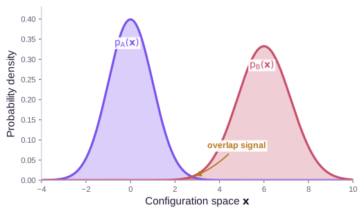
The core problem is to bridge A and B without requiring direct overlap between their equilibrium distributions. AIS supplies that bridge.

---

Part 2: The AIS Framework

AIS (Neal, 2001) fixes the overlap problem from direct free-energy comparison by bridging states A and B through intermediate distributions. Neighboring distributions overlap even when the endpoints do not. The resulting forward and reverse path measures yield three identities; in the physics specialization, these become Jarzynski’s equality, Crooks’ fluctuation theorem, and the second law.

The AIS Setup

AIS bridges two distributions by constructing intermediates \(\hat{p}_0, \hat{p}_1, \ldots, \hat{p}_K\) — unnormalized densities with unknown normalizing constants \(Z_k\). The forward chain works as follows:

1. Draw \(\mathbf{x}_0 \sim p_0 = \hat{p}_0 / Z_0\).
2. For \(k = 1, \ldots, K\): apply an MCMC transition \(T_k(\mathbf{x}_k \mid \mathbf{x}_{k-1})\) that leaves \(p_k\) invariant.
3. Record the log importance weight:

\[\log w = \sum_{k=0}^{K-1} \bigl[\log \hat{p}_{k+1}(\mathbf{x}_k) - \log \hat{p}_k(\mathbf{x}_k)\bigr]\]

Two runs give different weights because each MCMC chain follows a different random path — \(w\) is a random variable. With many intermediates (slow annealing), each density ratio is close to 1 and \(\log w\) clusters tightly around \(\log(Z_K/Z_0)\). With few intermediates (fast annealing), the ratios fluctuate wildly and the estimate degrades.

Forward and Reverse Path Measures

The forward path measure is the joint probability of the entire chain \((\mathbf{x}_0, \ldots, \mathbf{x}_K)\):

\[\mathcal{P}_F[\mathbf{x}_0, \ldots, \mathbf{x}_K] = p_0(\mathbf{x}_0) \prod_{k=1}^{K} T_k(\mathbf{x}_k \mid \mathbf{x}_{k-1})\]

The reverse path measure starts from \(p_K\) and steps backward:

\[\mathcal{P}_R[\mathbf{x}_0, \ldots, \mathbf{x}_K] = p_K(\mathbf{x}_K) \prod_{k=1}^{K} \tilde{T}_k(\mathbf{x}_{k-1} \mid \mathbf{x}_k)\]

where \(\tilde{T}_k\) is the time-reversal of \(T_k\) under \(p_k\): if \(T_k\) satisfies detailed balance with respect to \(p_k\), then \(p_k(\mathbf{x}) T_k(\mathbf{y} \mid \mathbf{x}) = p_k(\mathbf{y}) \tilde{T}_k(\mathbf{x} \mid \mathbf{y})\).

The Path Measure Ratio

The log-ratio decomposes as:

\[\ln \frac{\mathcal{P}_F}{\mathcal{P}_R} = \ln \frac{p_0(\mathbf{x}_0)}{p_K(\mathbf{x}_K)} + \sum_{k=1}^{K} \ln \frac{T_k(\mathbf{x}_k \mid \mathbf{x}_{k-1})}{\tilde{T}_k(\mathbf{x}_{k-1} \mid \mathbf{x}_k)}\]

Detailed balance gives \(\ln \frac{T_k(\mathbf{x}_k \mid \mathbf{x}_{k-1})}{\tilde{T}_k(\mathbf{x}_{k-1} \mid \mathbf{x}_k)} = \ln p_k(\mathbf{x}_k) - \ln p_k(\mathbf{x}_{k-1})\). Substituting:

\[\ln \frac{\mathcal{P}_F}{\mathcal{P}_R} = \ln p_0(\mathbf{x}_0) - \ln p_K(\mathbf{x}_K) + \sum_{k=1}^{K} \bigl[\ln p_k(\mathbf{x}_k) - \ln p_k(\mathbf{x}_{k-1})\bigr]\]

The MCMC kernels have cancelled completely — the ratio depends only on the densities \(p_k\), not the transition kernels \(T_k\).

The sum telescopes when we group terms by sample point. Each \(\mathbf{x}_j\) contributes \(+\ln p_j(\mathbf{x}_j)\) from the \(k=j\) term and \(-\ln p_{j+1}(\mathbf{x}_j)\) from the \(k=j+1\) term:

\[\ln \frac{\mathcal{P}_F}{\mathcal{P}_R} = -\sum_{k=0}^{K-1} \bigl[\ln p_{k+1}(\mathbf{x}_k) - \ln p_k(\mathbf{x}_k)\bigr]\]

Writing \(\ln p_k = \ln \hat{p}_k - \ln Z_k\) and recognizing the importance weight:

Path measure ratio.

\[\log \frac{\mathcal{P}_F}{\mathcal{P}_R} = \log \frac{Z_K}{Z_0} - \log w\]

The MCMC kernels cancel (detailed balance), and the path measure ratio depends only on the importance weight \(w\) and the normalizing constant ratio \(Z_K / Z_0\). (All logs in Part 2 are natural logarithms.)

Unbiasedness of AIS

From \(\mathcal{P}_R / \mathcal{P}_F = w / (Z_K/Z_0)\), sum over all trajectories weighted by \(\mathcal{P}_F\):

\[\left\langle \frac{\mathcal{P}_R}{\mathcal{P}_F} \right\rangle_F = \sum_{\text{traj}} \mathcal{P}_R = 1\] \[\left\langle \frac{w}{Z_K/Z_0} \right\rangle_F = 1\]

Unbiasedness of AIS.

\[\langle w \rangle_F = \frac{Z_K}{Z_0}\]

The average importance weight over forward chains is exactly the normalizing constant ratio — regardless of the number of intermediates \(K\) or the quality of the MCMC transitions.

This is the central guarantee behind AIS: the estimator is unbiased for any annealing schedule.

The ELBO and Its Gap

Taking logs and applying Jensen’s inequality (\(\log \langle w \rangle \geq \langle \log w \rangle\)):

\[\langle \log w \rangle_F \leq \log \frac{Z_K}{Z_0}\]

The left side is the ELBO — the evidence lower bound. The gap has an information-theoretic interpretation:

ELBO gap = KL divergence.

\[\log \frac{Z_K}{Z_0} - \langle \log w \rangle_F = D_{\text{KL}}(\mathcal{P}_F \| \mathcal{P}_R)\]

The gap between the true log-normalizing-constant ratio and the ELBO equals the KL divergence between forward and reverse path measures. The bound is tight if and only if \(\mathcal{P}_F = \mathcal{P}_R\).

This follows directly: \(D_{\text{KL}}(\mathcal{P}_F \| \mathcal{P}_R) = \langle \log(\mathcal{P}_F / \mathcal{P}_R) \rangle_F = \log(Z_K/Z_0) - \langle \log w \rangle_F\).

The Jensen bound is tight only when \(\log w\) is constant across trajectories, so every chain produces the same weight. This requires the chain to equilibrate at each intermediate distribution before moving to the next, which means infinite MCMC steps per level. With fewer steps, forward and reverse chains diverge, the KL grows, and the ELBO loosens.

The variance problem. With too few intermediates, most chains have \(w \ll Z_K/Z_0\), and rare ones with \(w \gg Z_K/Z_0\) dominate the average. The estimator is unbiased but has exponentially large variance — Zwanzig’s overlap problem from Part 1, transferred from configuration space to trajectory space.

---

Part 3: Non-Equilibrium Processes and Work

Non-equilibrium physics is a special case of the AIS identities: choose Boltzmann intermediates along a protocol and Langevin dynamics as the transition kernel. This specialization turns the log importance weight into work, and the same path-measure ratio becomes the thermodynamic identities derived in the Non-Equilibrium Equalities section.

Intermediates = Boltzmann distributions along a protocol. Define a protocol parameter \(\lambda_k\) interpolating from \(\lambda_0 = 0\) (state A) to \(\lambda_K = 1\) (state B), with:

\[\hat{p}_k(\mathbf{x}) = e^{-\beta U(\mathbf{x}, \lambda_k)}, \qquad U(\mathbf{x}, \lambda) = (1 - \lambda) U_A(\mathbf{x}) + \lambda \, U_B(\mathbf{x})\]

MCMC = Langevin dynamics. At each step, the particle slides downhill on the current potential and receives a random thermal kick:

\[\mathbf{x}_{k+1} = \mathbf{x}_k - \nabla U(\mathbf{x}_k, \lambda_k) \Delta t + \sqrt{2/\beta} \, \boldsymbol{\xi}_k, \qquad \boldsymbol{\xi}_k \sim \mathcal{N}(0, \Delta t \, \mathbf{I})\]

The importance weight becomes work. With the distributions and dynamics specified, we can evaluate the per-step log-density ratio from Part 2 in this physical setting:

\[\log \hat{p}_{k+1}(\mathbf{x}_k) - \log \hat{p}_k(\mathbf{x}_k) = -\beta\bigl[U(\mathbf{x}_k, \lambda_{k+1}) - U(\mathbf{x}_k, \lambda_k)\bigr]\]

So \(\log w = -\beta \sum_{k=0}^{K-1} [U(\mathbf{x}_k, \lambda_{k+1}) - U(\mathbf{x}_k, \lambda_k)]\). Physicists call this sum the work:

Work (discrete).

\[W = \sum_{k=0}^{K-1} \bigl[U(\mathbf{x}_k, \lambda_{k+1}) - U(\mathbf{x}_k, \lambda_k)\bigr]\]

The total change in potential energy due to protocol steps, evaluated at the current configuration. Each term is the energy cost of shifting the potential from \(\lambda_k\) to \(\lambda_{k+1}\) while the particle sits at \(\mathbf{x}_k\). The importance weight is \(w = e^{-\beta W}\).

For the linear interpolation, \(U(\mathbf{x}, \lambda_{k+1}) - U(\mathbf{x}, \lambda_k) = \Delta\lambda_k \cdot [U_B(\mathbf{x}) - U_A(\mathbf{x})]\): the work at each step is the energy difference between B and A, scaled by the protocol step size.

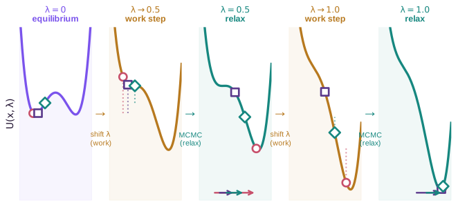
Now run many independent copies. Each receives different noise, producing different trajectories and different work values:

• Lucky run (low work, high \(w\)). The sample lands in a high-density region of \(p_{k+1}\) before the distribution shifts much — per-step ratios are close to 1, \(\log w\) stays near \(\log(Z_K/Z_0)\), and work \(W\) is close to \(\Delta F\).
• Unlucky run (high work, low \(w\)). The chain gets trapped in a mode of \(p_k\) with low density under \(p_{k+1}\) — each step gives a large negative density ratio, \(\log w\) falls far below \(\log(Z_K/Z_0)\), and work \(W\) far exceeds \(\Delta F\).

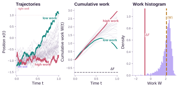
Quasistatic vs. driven processes. How fast we run the protocol determines the variance of \(W\):

• Quasistatic (\(K \to \infty\)): The chain equilibrates at every level. Every trajectory gives \(W = \Delta F\) (equivalently, all weights \(w\) are equal). Variance is zero, but cost is infinite.
• Driven (finite \(K\)): The chain cannot keep up. On average \(\langle W \rangle > \Delta F\); the excess is the dissipated work \(\langle W_{\text{diss}} \rangle = \langle W \rangle - \Delta F\). In AIS terms, it is the gap between the ELBO and the true \(\log(Z_K/Z_0)\).

Notation bridge. The two notational systems used throughout this post map as follows:

AIS (Part 2)	Physics (this section onward)
Unnormalized density \(\hat{p}_k\)	Boltzmann factor \(e^{-\beta U(\mathbf{x}, \lambda_k)}\)
Log importance weight \(\ln w\)	\(-\beta W\) (negative work times inverse temperature)
Log normalizing constant ratio \(\ln(Z_K/Z_0)\)	\(-\beta \Delta F\) (negative free energy difference)
Path measure ratio \(\ln(Z_K/Z_0) - \ln w\)	\(\beta(W - \Delta F)\)

The AIS identities become physics. The path measure ratio \(\ln(\mathcal{P}_F / \mathcal{P}_R) = \ln(Z_K/Z_0) - \ln w\) becomes \(\beta(W - \Delta F)\), where \(\Delta F = -(1/\beta)\ln(Z_K/Z_0)\) is the free energy difference. The three AIS identities from Part 2 now have direct physical names:

AIS identity	Physics name	Statement
Unbiasedness: \(\langle w \rangle = Z_K/Z_0\)	Jarzynski’s equality	\(\langle e^{-\beta W} \rangle = e^{-\beta \Delta F}\)
ELBO: \(\langle \log w \rangle \leq \log(Z_K/Z_0)\)	Second law	\(\langle W \rangle \geq \Delta F\)
ELBO gap = KL	Dissipation = KL	\(\langle W \rangle - \Delta F = (1/\beta) \, D_{\text{KL}}(\mathcal{P}_F | \mathcal{P}_R)\)

The path measure ratio contains more than expectations: it relates the full distribution of \(W\) under the forward and reverse processes. This is Crooks’ fluctuation theorem, the strongest of the three results, developed fully in Part 5.

---

Part 4: Continuous-Time Machinery

Discrete chains are enough for AIS, but Langevin dynamics live in continuous time. To carry the same path-measure ratio to SDEs, we need path integrals, Radon-Nikodym derivatives, Girsanov’s theorem, and forward-backward SDEs.

AIS introduced path measures in discrete time — products of MCMC kernels over finite chains. But continuous-time dynamics, such as the Langevin SDE, produce trajectories in \(C([0, T]; \mathbb{R}^d)\), where the discrete product formula no longer applies. We need a continuous-time theory of path measures.³

AIS parallel: This is the distribution over entire AIS chains from Part 2 — now extended to continuous time.

The Path Integral Picture

Physicists often describe path measures through the Feynman-Kac path integral. Consider a particle diffusing in a time-dependent potential \(U(\mathbf{x}, \lambda(t))\). The probability of observing a specific trajectory \(\mathbf{x}(\cdot)\) is weighted by an exponential of the action along that path:

\[\mathcal{P}[\mathbf{x}(\cdot)] \propto \exp\left(-\frac{\beta}{4} \int_0^T \lvert \dot{\mathbf{x}}(t) + \nabla U(\mathbf{x}(t), \lambda(t)) \rvert^2 \, dt\right)\]

This is the Onsager-Machlup action for overdamped Langevin dynamics. Each trajectory gets a weight determined by how “surprising” it is: trajectories that follow the force field (\(\dot{\mathbf{x}} \approx -\nabla U\)) have low action and high weight, while trajectories that fight the forces have high action and low weight.⁴

Discrete derivation of the Onsager-Machlup action. To see where this comes from, discretize time into \(N\) steps of size \(\Delta t\). At each step, the Langevin SDE says \(\mathbf{x}_{k+1} = \mathbf{x}_k - \nabla U_k \Delta t + \sqrt{2/\beta} \, \boldsymbol{\xi}_k\) where \(\boldsymbol{\xi}_k \sim \mathcal{N}(0, \Delta t \, \mathbf{I})\). The transition probability is Gaussian:

\[P(\mathbf{x}_{k+1} \mid \mathbf{x}_k) \propto \exp\left(-\frac{\beta}{4 \Delta t} \lvert \mathbf{x}_{k+1} - \mathbf{x}_k + \nabla U_k \Delta t \rvert^2\right)\]

The full path probability is the product over all steps:

\[\mathcal{P}_F[\mathbf{x}_0, \ldots, \mathbf{x}_N] = p_A(\mathbf{x}_0) \cdot \prod_{k=0}^{N-1} P(\mathbf{x}_{k+1} \mid \mathbf{x}_k)\]

Substituting the Gaussian form and collecting the exponents:

\[\propto p_A(\mathbf{x}_0) \cdot \exp\left(-\frac{\beta}{4\Delta t} \sum_{k=0}^{N-1} \lvert \Delta \mathbf{x}_k + \nabla U_k \Delta t \rvert^2\right)\]

In the continuous limit (\(N \to \infty\), \(\Delta t \to 0\)), the discrete sum \(\frac{\beta}{4\Delta t} \sum_k \lvert \Delta\mathbf{x}_k + \nabla U_k \Delta t \rvert^2\) becomes \(\frac{\beta}{4}\int_0^T \lvert \dot{\mathbf{x}} + \nabla U \rvert^2 dt\), the Onsager-Machlup action (equivalently \(\frac{1}{2\sigma^2}\int\) with \(\sigma^2 = 2/\beta\)). The discrete version is what we actually compute; the continuous version is formal notation.

AIS parallel: The Gaussian kernel above is the Langevin specialization of the generic MCMC kernel \(T_k\) from Part 2.

The path integral picture gives us a way to assign weights to individual trajectories. But Jarzynski and Crooks require the ratio of weights between the forward process (A \(\to\) B) and the reverse process (B \(\to\) A). Computing this ratio rigorously requires tools beyond the path integral: Radon-Nikodym derivatives and Girsanov’s theorem.

Why the Path Integral Picture Is Not Enough

The path integral formula \(\mathcal{P}[\mathbf{x}(\cdot)] \propto \exp(-\text{action})\) is useful but not rigorous: there is no uniform measure on continuous path space. In finite dimensions, \(p(x) \propto e^{-U(x)}\) makes sense because Lebesgue measure provides the reference. On \(C([0, T]; \mathbb{R}^d)\), no such flat reference exists — the path integral \(\int \mathcal{D}[\mathbf{x}(\cdot)]\) is formal notation, not a well-defined integral.⁵

The rigorous approach is to avoid writing an individual path measure’s density and work only with ratios between path measures. This ratio is the Radon-Nikodym derivative.

Radon-Nikodym Derivatives: The Right Way to Compare Path Measures

Individual path measures have no density with respect to a flat reference, but two path measures that share the same noise structure do have well-defined densities with respect to each other. This is the same idea as importance sampling: we don’t need \(p(x)\) and \(q(x)\) individually — we need their ratio \(p(x)/q(x)\).

Given two probability measures \(\mathbb{P}\) and \(\mathbb{Q}\) on the same space, the Radon-Nikodym derivative \(d\mathbb{P}/d\mathbb{Q}\) is the density of \(\mathbb{P}\) with respect to \(\mathbb{Q}\) — the function that reweights \(\mathbb{Q}\)-samples to produce \(\mathbb{P}\)-expectations:

\[\mathbb{E}_{\mathbb{P}}[f(X)] = \mathbb{E}_{\mathbb{Q}}\left[\frac{d\mathbb{P}}{d\mathbb{Q}}(X) \cdot f(X)\right]\]

For distributions on \(\mathbb{R}^d\), this is just the likelihood ratio \(p(x)/q(x)\). For path measures — distributions on \(C([0, T]; \mathbb{R}^d)\) — the Radon-Nikodym derivative is a functional of the entire trajectory. It is well-defined whenever the two processes share the same diffusion coefficient (same noise), even though neither process has a “density” in isolation.⁶

AIS parallel: The discrete version is the importance weight ratio from Part 2 — the continuous stochastic integral here is its rigorous counterpart.

Girsanov’s Theorem: Change of Measure for SDEs

Girsanov’s theorem solves this problem for diffusion processes. Consider two SDEs with the same noise but different drifts:

\[dX_t = a(X_t, t) \, dt + \sigma \, dW_t \qquad \text{vs.} \qquad dX_t = \tilde{a}(X_t, t) \, dt + \sigma \, dW_t\]

Girsanov’s theorem states that the Radon-Nikodym derivative between their path measures is:

Girsanov’s theorem (one direction).

\[\ln \frac{d\mathbb{P}^a}{d\mathbb{P}^{\tilde{a}}}(X) = \frac{1}{\sigma^2} \int_0^T (a_t - \tilde{a}_t)(X_t) \cdot dX_t - \frac{1}{2\sigma^2} \int_0^T \lvert a_t - \tilde{a}_t \rvert^2(X_t) \, dt\]

The first term is a stochastic integral (the “martingale part”); the second is a deterministic correction. Girsanov requires the diffusion coefficient \(\sigma\) to be the same for both processes: it changes the drift, not the noise. The noise cancels in the forward/reverse ratio because both processes have the same \(\sigma\).

A full proof uses exponential martingales, Novikov’s condition, and absolute continuity on path space. See Øksendal (Chapter 8) or Revuz & Yor (Chapter VIII) for the full treatment. In practice, the discrete derivation below verifies the result step by step; the theorem justifies taking the continuous limit.

Discrete Derivation of Girsanov’s Formula

Discretize both SDEs with Euler-Maruyama (step size \(\Delta t\)). Both processes share the same Gaussian noise — they differ only in the drift. The transition kernel for the first process is:

\[P^a(\mathbf{x}_{k+1} \mid \mathbf{x}_k) \propto \exp\left(-\frac{1}{2\sigma^2 \Delta t} \lvert \mathbf{x}_{k+1} - \mathbf{x}_k - a_k \Delta t \rvert^2\right)\]

and similarly for \(P^{\tilde{a}}\) with \(\tilde{a}_k\) replacing \(a_k\). The log-ratio at step \(k\) is:

\[\ln \frac{P^a(\mathbf{x}_{k+1} \mid \mathbf{x}_k)}{P^{\tilde{a}}(\mathbf{x}_{k+1} \mid \mathbf{x}_k)} = -\frac{1}{2\sigma^2 \Delta t}\left[\lvert \Delta\mathbf{x}_k - a_k \Delta t \rvert^2 - \lvert \Delta\mathbf{x}_k - \tilde{a}_k \Delta t \rvert^2\right]\]

where \(\Delta\mathbf{x}_k = \mathbf{x}_{k+1} - \mathbf{x}_k\). Expanding both squares, the \(\lvert \Delta\mathbf{x}_k \rvert^2\) terms cancel (same noise). What remains:

\[= \frac{1}{\sigma^2}(a_k - \tilde{a}_k) \cdot \Delta\mathbf{x}_k - \frac{1}{2\sigma^2}\lvert a_k - \tilde{a}_k \rvert^2 \Delta t\]

Summing over all steps and taking the continuous limit:

\[\ln \frac{d\mathbb{P}^a}{d\mathbb{P}^{\tilde{a}}}(X) = \frac{1}{\sigma^2} \int_0^T (a_t - \tilde{a}_t) \cdot dX_t - \frac{1}{2\sigma^2} \int_0^T \lvert a_t - \tilde{a}_t \rvert^2 \, dt\]

This reproduces Girsanov’s formula exactly. The discrete sum \(\sum_k (a_k - \tilde{a}_k) \cdot \Delta\mathbf{x}_k\) becomes the stochastic integral (an Itô integral, since the integrand is evaluated at the left endpoint \(\mathbf{x}_k\)); the sum \(\sum_k \lvert a_k - \tilde{a}_k \rvert^2 \Delta t\) becomes the deterministic correction.

AIS parallel: For two Langevin chains with different drifts, the discrete log importance weight is a sum of drift-difference terms at each step — the discrete Girsanov formula.

Girsanov compares two forward processes, SDEs running in the same direction with different drifts. The remaining step is to handle processes running in opposite directions.

Forward-Backward SDEs

Girsanov’s theorem compares two processes running in the same direction — two forward SDEs with different drifts. But we need to compare processes running in opposite directions: the forward protocol (A \(\to\) B) against the reverse protocol (B \(\to\) A). This requires pairing a forward Itô SDE with a backward Itô SDE, which introduces a new notational distinction (forward vs. backward integration). We adopt the notation from Vargas et al., 2024:

Forward-backward SDEs.

\[d X_t = a(X_t, t) \, dt + \sigma \, \fwd{d} W_t, \qquad X_0 \sim \mu \qquad \Rightarrow \qquad X \sim \fwd{\mathbb{P}}^{\mu, a}\] \[d X_t = b(X_t, t) \, dt + \sigma \, \bwd{d} W_t, \qquad X_T \sim \nu \qquad \Rightarrow \qquad X \sim \bwd{\mathbb{P}}^{\nu, b}\]

where \(\fwd{d} W_t\) and \(\bwd{d} W_t\) denote forward and backward Itô integration (see the Fokker-Planck post for definitions of Itô calculus and stochastic integrals), and \(\fwd{\mathbb{P}}^{\mu, a}\), \(\bwd{\mathbb{P}}^{\nu, b}\) are the associated path measures on \(C([0, T]; \mathbb{R}^d)\).

The forward SDE generates trajectories from \(\mu\) at time 0; the backward SDE generates trajectories from \(\nu\) at time \(T\). For the physics setting, \(a_t = \frac{\sigma^2}{2} \nabla \log \pi_t = -\nabla U_t\) with \(\pi_t\) interpolating from \(\pi_0\) to \(\pi_T\) — exactly the non-equilibrium protocol from Part 3. For diffusion models, \(a_t\) is the noising drift and \(b_t\) is the learned denoising drift.

Discrete-time counterpart. Discretizing the forward SDE with step size \(\Delta t\) gives the Euler-Maruyama chain:

\[\mathbf{x}_{k+1} = \mathbf{x}_k + a(\mathbf{x}_k, t_k) \Delta t + \sigma \boldsymbol{\xi}_k, \qquad \boldsymbol{\xi}_k \sim \mathcal{N}(0, \Delta t \, \mathbf{I})\]

with path measure \(\fwd{\mathbb{P}}^{\mu, a}[\mathbf{x}_0, \ldots, \mathbf{x}_N] = \mu(\mathbf{x}_0) \cdot \prod_k P(\mathbf{x}_{k+1} \mid \mathbf{x}_k)\). The backward SDE discretizes analogously, starting from \(\mathbf{x}_N \sim \nu\) and stepping in reverse:

\[\mathbf{x}_{k} = \mathbf{x}_{k+1} + b(\mathbf{x}_{k+1}, t_k) \Delta t + \sigma \boldsymbol{\xi}_k\]

with path measure \(\bwd{\mathbb{P}}^{\nu, b}[\mathbf{x}_0, \ldots, \mathbf{x}_N] = \nu(\mathbf{x}_N) \cdot \prod_k P_R(\mathbf{x}_k \mid \mathbf{x}_{k+1})\). The reverse transition \(P_R(\mathbf{x}_k \mid \mathbf{x}_{k+1})\) is a Gaussian centered at \(\mathbf{x}_{k+1} + b(\mathbf{x}_{k+1}, t_k) \Delta t\) — the same noise variance, but the drift is evaluated at \(\mathbf{x}_{k+1}\) and pushes backward. This is the reverse kernel used in the discrete derivation in Part 2.

AIS parallel: The forward-backward SDE pair is the continuous-time version of the forward and reverse AIS chains from Part 2. The Euler-Maruyama kernel is one specific MCMC choice; the importance weight \(w = \mathcal{P}_F / \mathcal{P}_R\) is the Radon-Nikodym derivative.

The Forward-Backward Radon-Nikodym Derivative

The remaining object is the log-ratio between the forward and backward path measures. Vargas et al. (2024, Proposition 2.2) give it as:

Forward-backward Radon-Nikodym derivative. Given a reference path measure \(\fwd{\mathbb{P}}^{\Gamma_0, \gamma^+} = \bwd{\mathbb{P}}^{\Gamma_T, \gamma^-}\):

\[\ln \frac{d\fwd{\mathbb{P}}^{\mu, a}}{d\bwd{\mathbb{P}}^{\nu, b}}(X) = \ln \frac{d\mu}{d\Gamma_0}(X_0) - \ln \frac{d\nu}{d\Gamma_T}(X_T)\] \[\quad + \frac{1}{\sigma^2} \int_0^T (a_t - \gamma_t^+)(X_t) \cdot \left(\fwd{d}X_t - \frac{1}{2}(a_t + \gamma_t^+)(X_t) \, dt\right)\] \[\quad - \frac{1}{\sigma^2} \int_0^T (b_t - \gamma_t^-)(X_t) \cdot \left(\bwd{d}X_t - \frac{1}{2}(b_t + \gamma_t^-)(X_t) \, dt\right)\]

This generalizes Girsanov’s theorem. The proof applies Girsanov twice — once for the forward process, once for the backward — using the reference to bridge between them. The key insight is that the reference \((\Gamma_0, \gamma^\pm)\) can be chosen freely; different choices redistribute weight between boundary terms and path integrals, enabling different computational strategies.⁷

Nelson’s Relation: When the RND Is Trivial

Nelson’s relation characterizes when the forward-backward RND equals 1, meaning the two path measures are identical (Nelson, 1967):

Nelson’s relation. \(\fwd{\mathbb{P}}^{\mu, a} = \bwd{\mathbb{P}}^{\nu, b}\) if and only if \(\nu = \fwd{\mathbb{P}}^{\mu, a}_T\) and

\[b_t = a_t - \sigma^2 \nabla \log \rho_t^{\mu, a}, \qquad \forall \, t \in (0, T]\]

where \(\rho_t^{\mu, a}\) is the time-marginal density of the forward process.

This is the continuous-time analogue of detailed balance. When \(a_t = \frac{\sigma^2}{2} \nabla \log \pi_t\), the reverse drift is \(b_t = -\frac{\sigma^2}{2} \nabla \log \pi_t\). If \(\pi_t\) is the true marginal at time \(t\), the forward and reverse path measures coincide, so the process is reversible. In physics language, this is the quasistatic limit: the system stays in equilibrium at every instant, the work equals \(\Delta F\) exactly, and the RND is \(e^0 = 1\).

AIS parallel: Nelson’s relation holds when each MCMC transition in the AIS chain runs long enough to reach equilibrium at \(p_k\) before moving to \(p_{k+1}\). In practice, we use a single (or few) MCMC step(s) per level — the chain never equilibrates, the forward and reverse path measures diverge, and the importance weights compensate with high variance.

The Work Identity: Plugging in the Physics

We now plug the physics, potential \(U\), temperature \(\beta\), and protocol \(\lambda(t)\), into the general forward-backward RND and recover the identity \(\ln(\mathcal{P}_F / \mathcal{P}_R) = \beta(W - \Delta F)\). This is the continuous-time version of Part 2’s path measure ratio \(\ln(Z_K/Z_0) - \ln w\). The Stratonovich chain rule collapses the path integrals into the work functional, generalizing beyond any particular discretization.

We return to the physics notation from Parts 1–3. The two notation systems used in this post are the same objects:

Physics (Parts 1–3)	General (Part 4)	AIS (Part 2)
\(\mathcal{P}_F\)	\(\fwd{\mathbb{P}}^{\mu, a}\)	Forward chain distribution
\(\mathcal{P}_R\)	\(\bwd{\mathbb{P}}^{\nu, b}\)	Reverse chain distribution
\(U(\mathbf{x}, \lambda)\)	\(-\frac{\sigma^2}{2} \ln \hat{\pi}_t(\mathbf{x})\)	\(-\log \hat{p}_k(\mathbf{x})\)
\(\beta = 1/k_BT\)	\(2/\sigma^2\)	1 (absorbed into densities)
Work \(W\)	\(\int_0^T \frac{\partial U}{\partial \lambda} \dot{\lambda} \, dt\)	\(-\log w\)
\(\Delta F\)	\(-\frac{\sigma^2}{2} \ln(Z_T/Z_0)\)	\(-\log(Z_K/Z_0)\)

We specialize the forward-backward RND to the non-equilibrium physics setting. Recall from Part 3 the time-dependent potential \(U(\mathbf{x}, \lambda(t))\) with Boltzmann distribution \(\pi_t(\mathbf{x}) = e^{-\beta U(\mathbf{x}, \lambda(t))} / Z_t\). The forward SDE is overdamped Langevin under this potential, and the backward SDE reverses the drift:

\[\text{Forward:} \quad dX_t = -\nabla U(X_t, \lambda(t)) \, dt + \sqrt{2/\beta} \, \fwd{d}W_t, \qquad X_0 \sim \pi_0\] \[\text{Backward:} \quad dX_t = +\nabla U(X_t, \lambda(t)) \, dt + \sqrt{2/\beta} \, \bwd{d}W_t, \qquad X_T \sim \pi_T\]

with reference \(\Gamma_0 = \pi_0\), \(\Gamma_T = \pi_T\), \(\gamma^+ = \gamma^- = 0\). The Stratonovich chain rule applied to \(U(X_t, \lambda(t))\) causes the path integrals to telescope, leaving only the work and boundary terms. After cancellation (see the collapsible derivation below):

Path measure ratio (core identity, rigorous form).

\[\ln \frac{\mathcal{P}_F}{\mathcal{P}_R}(X) = -\beta \Delta F + \beta W[X]\]

where the work is \(W[X] = \int_0^T \frac{\partial U}{\partial \lambda}(X_t, \lambda(t)) \dot{\lambda}(t) \, dt\) and the free energy difference is \(\Delta F = F_T - F_0 = -\frac{1}{\beta} \ln \frac{Z_T}{Z_0}\).

The general forward-backward RND was given above. This work identity is the result of specializing it to the physics setting — choosing the specific drifts \(\pm \nabla U\) from the non-equilibrium protocol and using the Stratonovich chain rule to collapse the path integrals into the work functional \(W\) from Part 3.

Full rigorous derivation (click to expand)

Step 1: The Radon-Nikodym derivative via Stratonovich integral. Starting from the forward-backward RND formula above with reference \(\Gamma_0 = \pi_0\), \(\Gamma_T = \pi_T\), \(\gamma^+ = \gamma^- = 0\):

$$\ln \frac{\mathcal{P}_F}{\mathcal{P}_R}(X) = \ln \frac{\pi_0(X_0)}{\pi_T(X_T)} - \beta \int_0^T \nabla U(X_t, \lambda(t)) \circ dX_t$$

The Stratonovich form arises from combining the forward and backward Itô integrals. This step requires Girsanov's theorem to rigorously define the change of measure from the reference process to each SDE.

Step 2: Apply the Stratonovich chain rule to \(U(X_t, \lambda(t))\). The Stratonovich integral \(\circ dX_t\) preserves the ordinary chain rule from calculus — \(df(X_t) = f'(X_t) \circ dX_t\) — which is why the following telescoping works. (The Itô integral does not preserve the chain rule; it would add a correction term \(\frac{1}{2}\sigma^2 \Delta U\), which must then be tracked separately.) Applying the Stratonovich chain rule:

$$dU(X_t, \lambda(t)) = \nabla U \circ dX_t + \frac{\partial U}{\partial \lambda} \dot{\lambda} \, dt$$

Rearranging and integrating from \(0\) to \(T\):

$$-\beta \int_0^T \nabla U \circ dX_t = -\beta \bigl[U(X_T, \lambda_T) - U(X_0, \lambda_0)\bigr] + \beta \int_0^T \frac{\partial U}{\partial \lambda} \dot{\lambda} \, dt$$

The second term is \(\beta W\) — the work from Part 3.

Step 3: Combine and cancel. Substituting into Step 1 and using \(\pi_t = e^{-\beta U(\cdot, \lambda(t))}/Z_t\):

$$\ln \frac{\mathcal{P}_F}{\mathcal{P}_R}(X) = \underbrace{\ln \frac{\pi_0(X_0)}{\pi_T(X_T)}}_{-\beta U_0(X_0) + \beta U_T(X_T) + \ln(Z_T/Z_0)} \underbrace{- \beta[U_T(X_T) - U_0(X_0)]}_{\text{from chain rule}} + \beta W$$

The potential energy terms cancel exactly:

$$= \ln \frac{Z_T}{Z_0} + \beta W = -\beta \Delta F + \beta W = \beta(W - \Delta F)$$

∎

Why Stratonovich? The Stratonovich integral preserves the ordinary chain rule, which is why the telescoping in Step 2 works cleanly. Using the Itô integral instead would introduce an additional \(\frac{1}{2}\sigma^2 \Delta U\) correction term (the Itô-Stratonovich conversion), which must then be tracked and cancelled — possible but messier.

The continuous-time path measure ratio has the same form \(\beta(W - \Delta F)\) as the discrete AIS ratio \(\ln(Z_K/Z_0) - \ln w\) from Part 2, with \(\ln w = -\beta W\) and \(\Delta F = -(1/\beta)\ln(Z_K/Z_0)\). The continuous-time derivation adds no new equality. It provides the rigorous foundation for the discrete results and extends them beyond Euler-Maruyama to any discretization scheme that converges to the Langevin SDE. Part 5 now extracts the three named equalities from this identity.

---

Part 5: Non-Equilibrium Equalities

The discrete and continuous derivations give the same identity:

• Discrete (Part 2): \(\ln(\mathcal{P}_F / \mathcal{P}_R) = \ln(Z_K/Z_0) - \ln w\), from detailed balance cancellation in AIS chains.
• Continuous (Part 4): \(\ln(\mathcal{P}_F / \mathcal{P}_R) = \beta(W - \Delta F)\), from the Stratonovich chain rule applied to the Langevin SDE.

These are the same identity in different notation (\(\ln w = -\beta W\), \(\ln(Z_K/Z_0) = -\beta \Delta F\)). This part extracts the three named results that follow from it.

Jarzynski’s Equality

The derivation is the same as Part 2’s unbiasedness proof, now in physics notation. From \(\mathcal{P}_F / \mathcal{P}_R = e^{\beta(W - \Delta F)}\), integrating \(\mathcal{P}_R / \mathcal{P}_F\) against \(\mathcal{P}_F\) gives 1:

\[\left\langle e^{-\beta(W - \Delta F)} \right\rangle_F = 1\]

Jarzynski’s equality (Jarzynski, 1997).

\[\left\langle e^{-\beta W} \right\rangle_F = e^{-\beta \Delta F}\]

The exponential average of work over forward non-equilibrium trajectories gives the exact equilibrium free energy difference — regardless of protocol speed, number of steps, or how far from equilibrium the process is driven.

The equality has three useful consequences:

1. \(\Delta F\) is an equilibrium quantity. \(W\) is measured from non-equilibrium trajectories. The equality holds for any protocol.
2. The second law \(\langle W \rangle \geq \Delta F\) follows from Jensen’s inequality: \(e^{-\beta \Delta F} = \langle e^{-\beta W} \rangle \geq e^{-\beta \langle W \rangle}\).
3. The bound is tight only when \(W\) is constant — the quasistatic limit where every trajectory gives \(W = \Delta F\).

In AIS terms: \(\langle w \rangle = Z_K/Z_0\) (unbiasedness), \(\langle \log w \rangle \leq \log(Z_K/Z_0)\) (the ELBO), and the bound is tight when all importance weights are equal (perfect annealing).

The variance problem. This is the same overlap issue encountered in Parts 1 and 2, now in the work variable: rare low-work trajectories carry exponentially large weight, and the effective sample size collapses for fast protocols.

Crooks’ Fluctuation Theorem

The path measure ratio relates the entire distribution of work, not only its expectations. For a given work value \(W\), group all trajectories that produce that value:

Crooks’ fluctuation theorem (Crooks, 1999).

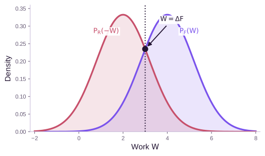
\[\frac{P_F(W)}{P_R(-W)} = e^{\beta(W - \Delta F)}\]

The ratio of the probability of observing work \(W\) in the forward direction to the probability of observing work \(-W\) in the reverse direction is exponentially related to how far \(W\) deviates from \(\Delta F\).

Crooks is stronger than Jarzynski: it relates the entire work distribution, rather than only an exponential average. Jarzynski is recovered by integrating both sides over \(W\).

Deriving Jarzynski from Crooks (click to expand)

Start from Crooks: \(P_F(W) = e^{\beta(W - \Delta F)} P_R(-W)\). Multiply both sides by \(e^{-\beta W}\) and integrate over all \(W\):

$$\int e^{-\beta W} P_F(W) \, dW = e^{-\beta \Delta F} \int P_R(-W) \, dW = e^{-\beta \Delta F}$$

The left side is \(\langle e^{-\beta W} \rangle_F\), giving Jarzynski's equality. ∎

Physical intuition. Trajectories where the forward work is less than \(\Delta F\) (the system “got lucky”) are exponentially rare, but they are exactly as probable as the corresponding reverse trajectories where the reverse work exceeds \(\Delta F\). The crossing point \(P_F(W) = P_R(-W)\) occurs at \(W = \Delta F\), giving a graphical method for estimating \(\Delta F\) — the Bennett acceptance ratio (BAR). Shirts et al. showed BAR is the minimum-variance estimator given samples from both directions (Shirts et al., 2003).

Dissipation as KL Divergence

From Jarzynski and Jensen, the second law gives \(\langle W \rangle_F \geq \Delta F\). The gap is the average dissipated work \(\langle W_{\text{diss}} \rangle = \langle W \rangle_F - \Delta F\). This gap has an information-theoretic interpretation:

Dissipated work as KL divergence.

\[\langle W_{\text{diss}} \rangle = \frac{1}{\beta} D_{\text{KL}}(\mathcal{P}_F \| \mathcal{P}_R)\]

The average work wasted beyond the free energy difference equals (up to temperature) the KL divergence between the forward and reverse path measures. Reversible processes (zero dissipation) have \(\mathcal{P}_F = \mathcal{P}_R\).

This is the ELBO gap identity from Part 2 in physics notation. The same information-geometric view also underlies thermodynamic metric and optimal-protocol results (Sivak & Crooks, 2012):

\[D_{\text{KL}}(\mathcal{P}_F \| \mathcal{P}_R) = \left\langle \ln \frac{\mathcal{P}_F}{\mathcal{P}_R} \right\rangle_F = \left\langle \beta(W - \Delta F) \right\rangle_F = \beta \langle W_{\text{diss}} \rangle\]

Irreversibility equals information loss, measured as KL divergence between forward and reverse path measures. A process with zero dissipation is perfectly reversible: every trajectory gives \(W = \Delta F\), the forward and reverse path measures coincide, and the KL vanishes. Any departure from reversibility, such as running the protocol too fast, using too few MCMC steps, or learning an imperfect score function, creates nonzero dissipation. For generative models, \(D_{\text{KL}}(\mathcal{P}_F \| \mathcal{P}_R)\) becomes a diagnostic for mismatch between the learned path measure and the target reverse path measure.

---

Part 6: Connections to Generative Models

The AIS-Jarzynski connection has been the throughline of this post since Part 2. The same path-measure language also helps read diffusion models and GFlowNets. A diffusion model has a forward noising path measure and a learned reverse denoising path measure; its variational loss can be read as a KL between those path measures. A GFlowNet (Bengio et al., 2021) has a forward construction path measure and a backward deconstruction path measure; trajectory balance (Malkin et al., 2022) asks their ratio to match the terminal reward up to the partition function.

The diagnostic is the same in all three cases: how different are the forward and reverse path measures? In AIS this appears as loose importance weights, in diffusion models as the gap between the learned reverse process and the true reverse process, and in GFlowNets as variance in the trajectory-balance log-ratio. The physics language turns several generative-model objectives into one question about reversibility and dissipation.

---

Closing

AIS, diffusion models, and GFlowNets all compare forward and reverse path measures. The identity \(\ln(\mathcal{P}_F / \mathcal{P}_R) = \beta(W - \Delta F)\) appears as an importance weight, a trajectory-balance condition, or a variational gap depending on the setting.

Ask what path distribution the algorithm samples and how far it is from the reverse or target path distribution. In physics this is dissipation. In ML it is transport efficiency.

---

References

• C. Jarzynski, “Nonequilibrium equality for free energy differences,” Physical Review Letters, 1997. DOI. ↩
• G. E. Crooks, “Entropy production fluctuation theorem and the nonequilibrium work relation for free energy differences,” Physical Review E, 1999. DOI. ↩
• R. M. Neal, “Annealed importance sampling,” Statistics and Computing, 2001. DOI. ↩
• R. W. Zwanzig, “High-temperature equation of state by a perturbation method,” Journal of Chemical Physics, 1954. DOI. ↩
• E. Nelson, Dynamical Theories of Brownian Motion, Princeton University Press, 1967. PDF. ↩
• M. R. Shirts, E. Bair, G. Hooker, and V. S. Pande, “Equilibrium free energies from nonequilibrium measurements using maximum-likelihood methods,” Physical Review Letters, 2003. DOI. ↩
• D. A. Sivak and G. E. Crooks, “Thermodynamic metrics and optimal paths,” Physical Review Letters, 2012. DOI. ↩
• F. Vargas, S. Padhy, D. Blessing, and N. Nüsken, “Transport meets variational inference: Controlled Monte Carlo Diffusions,” ICLR, 2024. ICLR 2024. ↩
• E. Bengio, M. Jain, M. Korablyov, D. Precup, and Y. Bengio, “Flow network based generative models for non-iterative diverse candidate generation,” NeurIPS, 2021. NeurIPS. ↩
• N. Malkin, M. Jain, E. Bengio, C. Sun, and Y. Bengio, “Trajectory balance: Improved credit assignment in GFlowNets,” NeurIPS, 2022. NeurIPS. ↩

---

Footnotes