On this page
Adapted from my 2025 Machine Learning for Molecules lectures. Molecular generation proposes chemical objects; reaction modeling asks how they can change or be made. This article follows the resulting distribution through constraints, route search, and experiments, while Discrete Flow and Generator Matching develops the underlying continuous-time machinery.
A Molecule Is Not an Arbitrary Graph
The usual statement of molecular generation sounds simple: learn a distribution \(p_\theta(G)\) from observed molecular graphs, then sample new graphs with desired properties. The difficulty is concentrated in the word graph. An image remains an image when a few pixels are wrong. A molecular graph can cease to describe a molecule when one bond is wrong, one charge is omitted, or one stereocenter is inverted.
Write a molecular graph as \(G=(V,E)\). Each node carries an atom type and possibly formal charge, aromaticity, or chirality. Each edge carries a bond type and possibly stereochemical information. Validity couples these labels. Neutral carbon and oxygen allow different valence patterns; aromatic bonds participate in rings; disconnected components may represent salts or reagents rather than one compound. A decoder that predicts each label accurately in isolation can still produce an inconsistent combination.
The representation also contains symmetries that the model should not mistake for chemical differences. Ethanol has an underlying heavy-atom graph \(\mathrm{C{-}C{-}O}\). It can be serialized as CCO or OCC, and its nodes can be indexed in six possible orders, but these choices do not create six molecules. For every node permutation \(\pi\), a graph distribution should satisfy
where \(\pi G\) consistently permutes the node and edge tensors. A string model encounters a related many-to-one problem because a molecule can have multiple valid SMILES strings. Canonicalization chooses one spelling; randomized SMILES exposes several spellings; neither changes the underlying chemical object.
I will use 2-fluoroethanol as a bookkeeping example. Its heavy-atom graph is the path
\[O_1-C_2-C_3-F_4,\]represented by strings such as OCCF and FCCO. The atom types and neighborhoods distinguish all four heavy atoms, so the labeled tensor has \(4!=24\) node indexings and a trivial automorphism group. More generally, if \(\operatorname{Aut}(G)\) is the set of node permutations that leave a labeled graph unchanged, the number of distinct tensor indexings is
The bracket \([G]\) denotes the equivalence class of all indexings of the same chemical graph. A model defined on indexed tensors induces a probability on the chemical object only after summing over that class:
\[p_\theta([G]) =\sum_{G'\in[G]}p_\theta(G').\]Exact permutation invariance makes every term equal, giving \(p_\theta([G])=24p_\theta(G)\) for this example. A model that assigns different probabilities to the 24 indexings has learned an arbitrary storage convention. Canonicalization avoids the sum by selecting one representative, but it also turns the canonicalizer into part of the data distribution. Randomized representations instead expose several representatives and leave the model or evaluator to marginalize them.
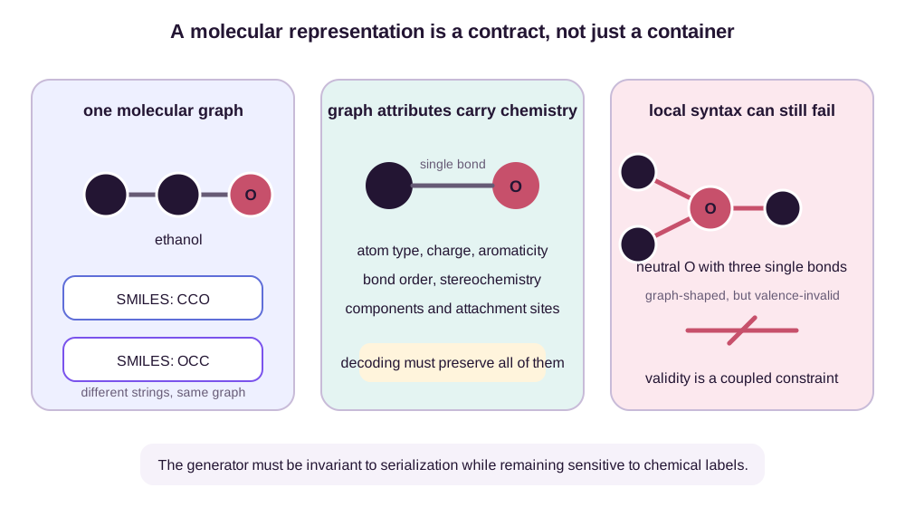
This tension drives architecture. Sequential models make constraints easier to check after every edit but introduce an arbitrary construction order. Parallel models respect permutation symmetry more naturally but must coordinate many node and edge decisions at once. Motif-based models move the constraint boundary again: they assemble larger valid pieces, at the cost of deciding in advance which pieces exist.
Autoregressive Generation Turns a Graph Into a History
An autoregressive generator chooses a sequence of actions \(a_1,\ldots,a_T\) such as add an atom, attach a bond, close a ring, or stop. Given an ordering \(\pi\), the chain rule gives
\[p_\theta(G,\pi) =\prod_{t=1}^{T}p_\theta(a_t\mid a_1,\ldots,a_{t-1}).\]The partial molecule is the state. Its advantage is immediate: an action grammar can mask choices that violate allowed valences or attachment rules. If the current carbon already has four bond-order units, another bond can be forbidden. Errors remain possible, but validity can be defended locally rather than repaired after a full adjacency matrix appears.
The price is that the model learns histories, not only graphs. The correct graph likelihood requires summing over all action sequences that produce it,
\[p_\theta(G)=\sum_{\pi\in\Pi(G)}p_\theta(G,\pi),\]which is usually intractable. Training therefore selects or samples an ordering. Breadth-first order shortens the range of edge decisions because a new node is likely to connect near the current frontier. It does not remove the ordering dependence. GraphRNN made this sequential node-and-edge decomposition explicit for general graph generation (You et al., 2018).
The sum changes a molecule probability even in a four-atom grammar. Suppose the grammar grows a path from either end and permits only two histories for 2-fluoroethanol. From the oxygen end, let the successive probabilities for choosing \(O\), attaching \(C\), attaching the second \(C\), attaching \(F\), and stopping be
\[(0.30,0.50,0.20,0.50,0.80).\]That history has probability
\[p_\theta(h_{O\to F}) =0.30\times0.50\times0.20\times0.50\times0.80 =0.012.\]Growing the same graph from the fluorine end might have action probabilities \((0.20,0.40,0.25,0.50,0.80)\), giving
\[p_\theta(h_{F\to O})=0.008.\]Under this restricted grammar, the graph probability is \(0.012+0.008=0.020\). Taking the more likely history would undercount it by \(40\%\); scoring only the canonical history would conflate a convention with chemical likelihood. Real graphs admit many more orders, ring-closure times, and equivalent attachment choices. Exact summation is then replaced by an ordering policy, importance sampling, or an objective that trains across randomized histories. Each replacement defines an approximation to the quotient probability, not an algebraic identity.
Construction order and node order are related but different equivalence relations. The same action history can be stored under multiple atom indexings, and the same indexed final graph can be reached by multiple action histories. A likelihood intended for chemical objects must marginalize both sources of multiplicity or state which representative it scores. The marginalization logic parallels the alternative-history sums in the Fokker–Planck chapter, although here the alternatives are discrete construction records rather than previous particle positions.
Autoregression also creates exposure bias. During training, the next action is conditioned on a correct partial graph. During sampling, it is conditioned on the model’s own earlier choices. An unlikely bond added at step 5 may force awkward actions at steps 6 through 20. Hard masks prevent some invalid paths, but they cannot recognize every unstable ring system, implausible functional-group combination, or poor synthetic decision.
Motif generation reduces the horizon by treating rings or functional fragments as larger tokens. A benzene ring can be added in one decision instead of six atom additions and six bond decisions. Junction-tree generation formalizes this idea by first building a tree of chemical substructures and then assembling the detailed molecular graph (Jin et al., 2018). The tradeoff is structural: a vocabulary that makes common chemistry easy can make genuinely new motifs unreachable. “Validity by construction” is always validity relative to the construction grammar.
Parallel Generation Moves the Burden to Joint Consistency
A one-shot graph generator predicts a node tensor and edge tensor together. A discrete diffusion model makes this prediction iterative: it corrupts categorical atom and bond labels, then learns to reverse the corruption. At a noisy step, each candidate edge may be absent, single, double, aromatic, or masked; each node may carry a noisy atom label. A permutation-equivariant network updates all of them without choosing a canonical node order.
Discrete state spaces matter here. Relaxing an adjacency matrix to continuous values can simplify optimization, but a value of \(0.4\) is not a chemical bond. The decoder eventually has to return to categorical decisions, where small continuous errors can change connectivity. Discrete denoising keeps the intermediate variables in the same categorical language as the output. DiGress is a representative construction: a Markov chain corrupts node and edge categories, and a graph transformer predicts the clean graph needed for reverse transitions (Vignac et al., 2023).
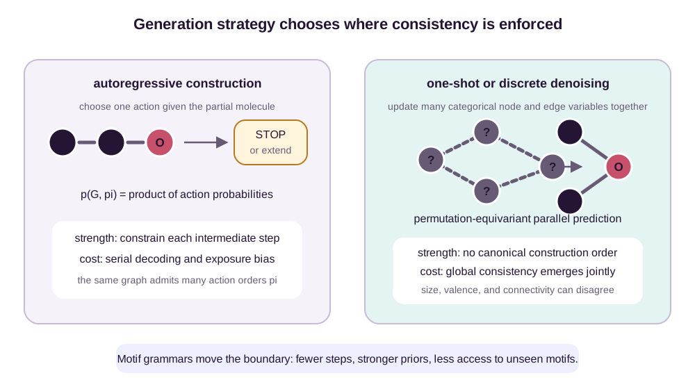
Parallel prediction does not automatically solve graph generation. The model still has to choose graph size or represent absent nodes, preserve symmetry while distinguishing atoms with different environments, and couple distant decisions such as ring closure. Independent edge logits may assign too many bonds to one atom. Enforcing valence after sampling can raise the validity rate while distorting the learned distribution: the postprocessor, not the model, decides which errors survive.
A five-outcome example makes the distortion visible. Suppose a parallel decoder assigns raw probability to three valid graphs and two invalid graphs:
| Raw proposal | Chemical status | Raw probability |
|---|---|---|
ethanol, CCO | valid | 0.35 |
dimethyl ether, COC | valid | 0.25 |
ethylene oxide, C1CO1 | valid | 0.15 |
| neutral oxygen with three single bonds | invalid valence | 0.15 |
| carbon with five single bonds | invalid valence | 0.10 |
Pure rejection accepts probability \(0.75\). Conditional on acceptance, the three valid probabilities become
\[(0.35,0.25,0.15)/0.75 =(0.467,0.333,0.200).\]The rejection sampler is exact for the raw model conditioned on this validity test, but that accepted distribution is not the raw model and need not equal the chemical target distribution. It also spends, on average, \(1/0.75=1.33\) proposals per accepted molecule.
A deterministic repair rule creates another distribution. Suppose repair removes the lowest-confidence bond: the overbonded oxygen maps to dimethyl ether, while the overbonded carbon maps to ethanol. All proposals now return a sanitized graph, but their probabilities are
\[p_{\mathrm{repair}} =(0.35+0.10,0.25+0.15,0.15) =(0.45,0.40,0.15).\]Relative to rejection, repair has moved \(6.7\) percentage points of mass toward dimethyl ether, \(5\) away from the ring, and \(1.7\) away from ethanol. The many-to-one projection creates collisions: an originally valid ether and a repaired invalid graph become indistinguishable. Reporting “100% valid after repair” discards the fact that \(25\%\) of raw samples were invalid and that the postprocessor reassigned their mass.
Hard action masks produce a third distribution. In the simplest terminal decision, masking the two invalid outcomes and renormalizing reproduces the rejection probabilities. But an autoregressive grammar may also forbid ring closure. Then ethylene oxide is unreachable, and the remaining probabilities renormalize to
\[(0.35,0.25)/(0.35+0.25)=(0.583,0.417),\]with zero mass on a valid mode. A mask can guarantee its encoded constraints exactly while excluding chemistry that the grammar forgot. Rejection, repair, and masking therefore answer different questions: condition the raw proposal, project it, or change its support before sampling.
The two paradigms therefore place the same difficulty in different locations. Autoregressive generation serializes a global constraint problem into locally checkable steps. Parallel generation preserves graph symmetry but asks the network and reverse process to coordinate global constraints. A useful comparison reports not only final validity and speed, but also how constraints were imposed, which failures were filtered, and whether filtering changed diversity.
Conditional Design Is More Than Adding a Property Label
Unconditional generation imitates a molecular dataset. Design asks for a conditional distribution \(p(G\mid\mathbf{y})\), where \(\mathbf{y}\) might contain solubility, binding affinity, band gap, toxicity, or a required scaffold. Conditioning can enter as an embedding supplied to every decoding step, as a conditional denoiser, or as guidance from a property predictor. Formally,
\[p(G\mid\mathbf{y})\propto p(\mathbf{y}\mid G)p(G).\]The prior \(p(G)\) keeps proposals near learned chemistry; the likelihood-like term rewards the requested property. Stronger guidance shifts probability toward the condition but can push the model outside the region where the property predictor is trustworthy.
A two-candidate calculation shows how quickly this can happen. Let the familiar candidate \(G_1\) be the 2-fluoroethanol graph above, with prior probability \(0.50\) and proxy likelihood \(p(y\mid G_1)=0.40\) for a hypothetical design condition. Let an unusual charged candidate \(G_2\) have prior \(0.05\) but proxy likelihood \(0.95\). With guidance strength \(\beta\), use the unnormalized score
\[w_\beta(G)=p(G)p(y\mid G)^\beta.\]At \(\beta=1\), the scores are \(0.200\) and \(0.0475\), so the prior keeps \(G_1\) ahead by a factor of \(4.21\). At \(\beta=5\), they become
\[w_5(G_1)=0.50(0.40)^5=0.00512, \qquad w_5(G_2)=0.05(0.95)^5\approx0.0387.\]The proxy-favored outlier is now \(7.56\) times more likely than the familiar molecule. This calculation does not say \(G_2\) is bad. It says the guided distribution is dominated by a likelihood surrogate precisely where the prior says data are sparse.
Predictive uncertainty can reverse the decision again. If the proxy reports predicted scores and standard deviations \((0.90,0.25)\) for \(G_2\) and \((0.70,0.05)\) for \(G_1\), a conservative score \(\mu-2\sigma\) ranks them as \(0.40\) and \(0.60\). The uncertainty penalty is still a learned heuristic; it is not a chemical guarantee. Calibration must be checked on the deployment population, especially after guidance changes that population.
Consider asking for high lipophilicity using a learned proxy. A generator may discover that extending hydrocarbon chains increases the score. It can then produce repetitive, insoluble molecules that satisfy the scalar proxy while violating the broader design intent. A binding predictor can be exploited through unusual charged groups or structures far from its training domain. Conditional success must therefore include uncertainty, domain of applicability, and competing properties—not merely the value of the optimized oracle.
Constraints also differ in kind. “Contains this scaffold” can often be enforced exactly by freezing a subgraph. “Has activity below 10 nM” is a noisy experimental claim mediated by a predictor. “Can be synthesized in three steps from available stock” requires a route, not a graph-local property. Treating all three as interchangeable conditioning vectors hides where evidence comes from.
An exact scaffold constraint is an indicator \(\mathbf{1}\{S\subseteq G\}\): candidates outside the allowed set receive zero probability if the decoder truly freezes the indexed subgraph and preserves its stereochemistry. A proxy constraint supplies only evidence about an unobserved measurement. A route constraint is existential—there must be at least one accepted sequence of reactions under a stated stock list and search budget. The first can be guaranteed by representation and actions. The latter two remain uncertain even when their model scores are high.
A Reaction Is a Small Edit Embedded in a Large Graph
Forward reaction prediction receives reactants and reagents and predicts products. Retrosynthesis reverses the question: given a desired product, propose precursor sets that could make it. These are not inverse functions. Several conditions can transform the same reactants into different products, and many precursor sets can lead to the same target.
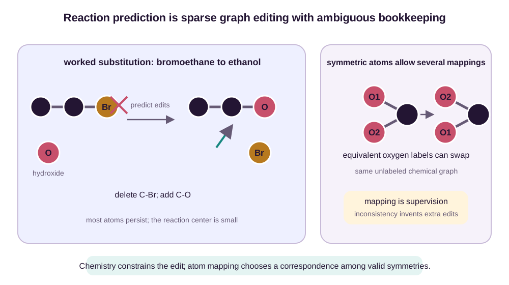
For many recorded single-step reactions, most atoms and bonds are unchanged. The transformation is concentrated in a small reaction center. This suggests an edit representation
\[G_{\mathrm{product}}=\operatorname{Apply}(G_{\mathrm{reactants}},\Delta),\]where \(\Delta\) contains bond deletions, bond additions, and bond-order changes. In a schematic nucleophilic substitution of bromoethane by hydroxide, the heavy-atom edit set deletes the carbon–bromine bond and adds a carbon–oxygen bond. Carbon skeleton atoms persist; the leaving group becomes a separate bromide component.
Index the bromoethane methyl carbon as \(C_1\), its bromine-bearing carbon as \(C_2\), bromine as \(Br_3\), and hydroxide oxygen as \(O_4\). With implicit hydrogens and unit bond order, the reactant edge set is
\[E_R=\{(1,2,1),(2,3,1)\},\]while \(O_4\) is a separate component. The product edge set for ethanol plus bromide is
\[E_P=\{(1,2,1),(2,4,1)\}.\]The sparse edit is therefore
\[\Delta^-=\{(2,3,1)\}, \qquad \Delta^+=\{(2,4,1)\}.\]If formal charges are explicit, the net record also changes \(O_4\) from \(-1\) to \(0\) and \(Br_3\) from \(0\) to \(-1\). Applying \(\Delta^-\) first yields a carbon center with an open valence; applying \(\Delta^+\) first yields a transient over-valent representation if hydrogens are not adjusted. The edit set describes the net recorded transformation, not an elementary mechanistic trajectory. A reaction model can rank this pair of bond edits without claiming that the dataset identifies transition states, solvent rearrangement, or the physical order of bond breaking and formation.
Template-based models store reaction patterns that specify a local environment and edit. Templates supply a strong chemical grammar and interpretable precedent, but their precision competes with coverage. A narrow pattern applies safely to few substrates; a broad pattern retrieves more cases but may ignore selectivity. Template-free graph models instead predict likely reaction centers, enumerate a small set of edited products, and rank them. This sparse-edit strategy avoids enumerating all possible product graphs; an early example learned reaction-center scores and ranked resulting candidates with a graph network (Jin et al., 2017).
Sequence models take another route: serialize reactants and products as SMILES and treat reaction prediction as translation. This removes explicit templates and can capture long-range context. The Molecular Transformer showed that attention-based sequence prediction could handle forward reactions and produce useful uncertainty estimates (Schwaller et al., 2019). Yet a syntactically fluent product can still violate atom conservation, choose the wrong stereoisomer, or omit a minor component. Graph edits and strings emphasize different structure; neither representation supplies missing conditions, yields, or experimental context.
Atom Mapping Is Necessary—and Not Unique
To learn edits, we need to know which reactant atom corresponds to which product atom. An atom mapping is a partial bijection between conserved atoms on the two sides. Once mapping is fixed, a bond present only on the reactant side is a deletion, and a bond present only on the product side is an addition.
But the chemical graph may admit automorphisms: permutations that leave it unchanged. In a carboxylate group, the two oxygen positions can be equivalent under resonance and symmetry at the level used by a dataset. Swapping their map numbers produces the same unlabeled structure but a different labeled correspondence. A mapping pipeline that makes inconsistent choices across examples can turn one chemical transformation into several apparent edit patterns. A model is then penalized for disagreeing with bookkeeping even when its product graph is correct.
Let \(\mathcal{M}(R,P)\) be the set of atom maps that produce the same reactant and product graphs under the evaluator’s equivalence rules. If a model assigns joint scores to a product and map, quotient-aware product likelihood sums the alternatives:
\[p_\theta([P]\mid R) =\sum_{m\in\mathcal{M}(R,P)}p_\theta(P,m\mid R).\]Suppose the two equivalent oxygen maps of a carboxylate receive probabilities \(0.60\) and \(0.30\), while chemically wrong products receive the remaining \(0.10\). A map-specific top-1 score credits only the chosen \(0.60\) correspondence. Product-level scoring credits \(0.90\) because the two maps describe the same accepted chemistry. The corresponding negative log scores are \(-\log0.60=0.511\) and \(-\log0.90=0.105\). Taking the maximum over maps is useful for top-1 equivalence, but it is not a normalized likelihood; the sum is the correct marginal when the map is latent.
Modern mapping systems can infer correspondences from reaction data without handcrafted reaction rules. Attention-derived mapping, for example, revealed that a reaction language model had learned atom correspondences implicitly (Schwaller et al., 2021). This is powerful preprocessing, but it should remain visible in evaluation. Report whether scoring compares mapped edits, canonicalized product graphs, or chemically equivalent products; these questions have different answers under symmetry.
Atom mapping can also leak the solution. If product-informed mappings or reaction-center labels are available to a model at test time, the task is no longer ordinary forward prediction from raw reactants. The safest pipeline separates information used to normalize training data from information the deployed model could actually observe.
The oxygen example shows the leakage mechanism. Before observing the product, reactant oxygens \(O_3\) and \(O_4\) are equivalent under the chosen graph representation. In a product ester, one oxygen is bonded to a new methyl carbon and the other is not. A mapper that sees both sides can choose the correspondence placing the product’s ester oxygen on \(O_3\). If those product-informed map numbers are then passed to a reaction-center predictor, the label “3” reveals which symmetric reactant atom receives the new bond. The model no longer has to infer that choice from reactants and conditions. A fair split must compute any map-derived feature without product access at deployment, or keep mapping strictly inside label construction and quotient the evaluation over equivalent answers.
Retrosynthesis Turns One Edit Into a Search Problem
A one-step retrosynthesis model proposes precursor sets for a target. A synthesis plan recursively applies such disconnections until every leaf is an available starting material. If each target has \(b\) plausible disconnections and a route has depth \(d\), naive enumeration grows like \(b^d\). The most accurate single-step predictor is not automatically the best planner: it may rank ten nearly identical disconnections highly while missing the one that leads to short, purchasable branches.
With \(b=12\) and \(d=4\), the terminal route count is
\[12^4=20{,}736.\]A budget of \(500\) node expansions cannot examine that tree exhaustively. Even a beam that retains the top five proposals at every depth still has \(5^4=625\) terminal route skeletons before accounting for convergent branches, protecting groups, or alternative suppliers. Search budget is therefore part of the route claim. “No route found” under 500 expansions means the policy and search failed within that budget; it does not prove that the molecule is unsynthesizable.
Planning therefore combines learned proposals with search. A policy prioritizes disconnections; a value or rollout estimate judges whether branches are likely to reach building blocks; filters reject implausible forward reactions. Neural-guided tree search demonstrated how learned reaction policies and symbolic search can work together for multistep planning (Segler et al., 2018).
The route is still a hypothesis. Patent datasets overrepresent successful reactions and often omit failed conditions. Reagent identity may be inconsistently separated from reactants. Yields from different laboratories are not directly comparable, and a step that works on milligram scale may fail at scale-up. A route with known reaction classes but unavailable starting materials is not actionable. Synthesis constraints should therefore enter generation early—through reaction-based construction, purchasable fragments, or route-aware objectives—rather than appear only as a final scalar penalty.
Step confidence also compounds at route level. Consider a three-step plan with estimated isolated yields \(0.80\), \(0.65\), and \(0.75\). Ignoring stoichiometric complications, its expected material fraction is
\[Y_{\mathrm{route}}=0.80\times0.65\times0.75=0.39.\]Under one-to-one stoichiometry, producing 100 mmol of target would require about \(100/0.39=256\) mmol of limiting starting material before additional losses or excess reagents. A two-step alternative at \(0.55\) yield per step gives \(0.55^2=0.3025\), so fewer steps do not automatically mean more product. Yield predictions are uncertain and correlated with scale, purification, and substrate context, but multiplying them exposes a fact that a per-step top-\(k\) metric hides: a sequence of individually plausible reactions can still be a low-throughput route.
Validity and Novelty Are the Beginning of Evaluation
Validity asks whether software can parse and sanitize a generated structure. Uniqueness asks whether samples repeat. Novelty asks whether they are absent from a reference set. These are necessary diagnostics, but each admits a weak solution. A model can generate many valid carbon chains, achieve high uniqueness through small substitutions, and appear novel because the training database is finite. None of this demonstrates useful chemical design.
Benchmarks such as GuacaMol expanded evaluation toward distribution matching and goal-directed, multi-objective tasks (Brown et al., 2019). A serious evaluation should continue further:
-
Canonicalize before counting. Different SMILES strings or atom orders should not inflate uniqueness and novelty. Near-duplicate scaffolds should be measured separately from exact duplicates.
-
Compare distributions, not only averages. Atom types, ring systems, scaffold frequencies, molecular sizes, and property distributions expose mode dropping that a mean score hides.
-
Audit conditional calibration. Measure success across requested property ranges, including hard or rare conditions, and use predictors that were not optimized jointly with the generator.
-
Respect reaction equivalence. Product accuracy should account for canonicalization, atom-mapping ambiguity, stereochemistry, and multiple plausible products. Retrosynthesis needs top-\(k\) precursor accuracy, diversity of disconnections, and route-level success.
-
Test synthesizability with routes. Heuristic synthetic-accessibility scores are cheap filters, not proofs. Route planners should use available building blocks and report search budget, route length, precedent, and forward-validation confidence.
-
Reserve the final claim for experiments. Predicted affinity, a plausible route, and a stable structure are evidence filters. Synthesis, characterization, and measured function are the test.
The denominators should follow one batch rather than appear as unrelated percentages. Consider a hypothetical run of \(1{,}000\) raw graphs:
| Stage | Survivors | Stage rate | Cumulative rate from raw |
|---|---|---|---|
| Sanitization succeeds | 820 | 820/1,000 = 82.0% | 82.0% |
| Canonically unique | 700 | 700/820 = 85.4% | 70.0% |
| Exactly novel to the reference set | 420 | 420/700 = 60.0% | 42.0% |
| Route found within the fixed search budget | 126 | 126/420 = 30.0% | 12.6% |
| Selected and ordered for synthesis | 24 | 24/126 = 19.0% | 2.4% |
| Synthesized and purified | 18 | 18/24 = 75.0% | 1.8% |
| Meets the measured property threshold | 5 | 5/18 = 27.8% | 0.5% |
Every row changes the population. The \(82\%\) sanitization rate refers to raw decoder outputs. The \(85.4\%\) uniqueness rate refers only to sanitized outputs, and its 120 collisions include repeated samples and alternative serializations. If both OCCF and FCCO appear, they count once after canonicalization. If 2-fluoroethanol already occurs in the reference set, our running candidate stops at the novelty row even if its proxy score was attractive. That is a correct rediscovery, not a novel design.
The route denominator is the 420 unique novel molecules submitted to the same planner with the same stock list and expansion budget. Only 126 receive a route under that contract. Selecting 24 for synthesis introduces another policy based on predicted property, route confidence, cost, and diversity. Eighteen purified products do not imply that six planned reactions were chemically impossible; failures may include procurement, reaction, workup, purification, or identity confirmation. Finally, five measured hits mean \(5/18=27.8\%\) of tested products and \(5/1000=0.5\%\) of raw proposals. Reporting only the first percentage makes the campaign look fifty-six times more productive than the end-to-end denominator.
The accepted batch is also not a sample from the original generator. It is distributed as
\[p_{\mathrm{selected}}(G) \propto p_\theta(G) \,a_{\mathrm{san}}(G) \,a_{\mathrm{novel}}(G) \,a_{\mathrm{route}}(G;B) \,a_{\mathrm{select}}(G),\]where \(B\) denotes the planner’s finite budget and stock database. Some factors are deterministic indicators; route and selection factors can be stochastic or policy-dependent. Measurement adds another missingness mechanism because only selected, successfully synthesized molecules are observed. The five measured hits estimate performance of this full adaptive pipeline, not unconditional accuracy over all 1,000 proposals.
Canonicalization is implicit in the chemical object \(G\) in this expression. Batch deduplication is not a per-molecule factor at all: whether a proposal survives depends on which equivalent proposal appeared first. That set-level dependence is another reason the final 24 candidates cannot be treated as independent samples from a simply reweighted generator.
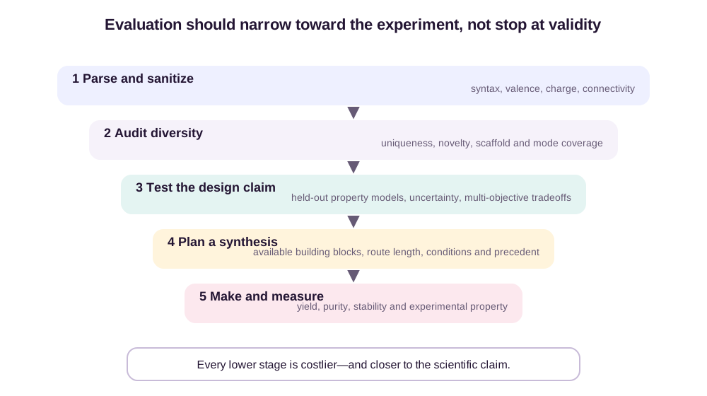
This final distinction matters because common objectives can disagree. Biasing generation toward structures that a planner can synthesize may reduce the best predicted property score. Gao and Coley showed that molecules favored by generative benchmarks can be difficult for synthesis planners and that synthetic-complexity bias trades against the primary objective (Gao & Coley, 2020). That is not an evaluation nuisance. It is the real multi-objective structure of molecular discovery.
Generation and Reaction Modeling Belong in One Loop
Molecular graph generation proposes what might exist. Reaction prediction asks how graphs transform. Retrosynthetic planning asks whether a sequence of those transformations reaches available matter. Keeping the tasks separate makes each benchmark cleaner, but it also creates the easiest failure mode in molecular AI: an impressive proposal with no credible path to a flask.
The durable abstraction is constrained structured prediction. The representation must quotient out irrelevant orderings while retaining charge, bond order, and stereochemistry. The generator must coordinate local valence with global connectivity. The reaction model must locate sparse edits without confusing atom-map bookkeeping for chemistry. The planner must turn plausible local steps into a globally feasible route. Evaluation must follow the same chain all the way to experiment.
The numerical examples above form one loop. Generation can assign 2-fluoroethanol probability through several serializations and construction histories, but canonicalization turns them into one molecule and novelty may remove it as a rediscovery. Guidance changes which candidates reach the planner; an exact scaffold mask and an uncertain activity proxy do not offer the same guarantee. The planner composes sparse transformations like the indexed bromoethane substitution, quotients equivalent atom maps, and searches only a small part of an exponential route tree. Synthesis and measurement then return outcomes on 24 deliberately selected candidates, not on an independent sample from the raw generator.
The next generation round should condition on what that loop actually observed. A failed sanitization diagnoses representation or decoding. Repeated canonical collisions diagnose mode concentration. Route-search failures can reflect either proposal chemistry or limited search. Synthesis failures update reaction and condition models only after recording where procurement, reaction, or purification failed. Measured property failures update the design oracle on the selected experimental population; correcting selection bias requires retaining the selection probabilities and negative results. Collapsing all failures into one reward discards the information needed to improve the responsible component.
The most useful molecular generator is therefore not the one that produces the largest number of novel valid graphs. It is the one whose proposals survive increasingly realistic constraints without collapsing to the training set—and whose failures remain legible enough to guide the next design cycle.
References
You, J., Ying, R., Ren, X., Hamilton, W., & Leskovec, J. (2018). GraphRNN: Generating Realistic Graphs with Deep Auto-regressive Models. Proceedings of the 35th International Conference on Machine Learning. ↩
Jin, W., Barzilay, R., & Jaakkola, T. (2018). Junction Tree Variational Autoencoder for Molecular Graph Generation. Proceedings of the 35th International Conference on Machine Learning. ↩
Vignac, C., Krawczuk, I., Siraudin, A., Wang, B., Cevher, V., & Frossard, P. (2023). DiGress: Discrete Denoising Diffusion for Graph Generation. International Conference on Learning Representations. ↩
Jin, W., Coley, C., Barzilay, R., & Jaakkola, T. (2017). Predicting Organic Reaction Outcomes with Weisfeiler–Lehman Network. Advances in Neural Information Processing Systems, 30. ↩
Schwaller, P., Laino, T., Gaudin, T., Bolgar, P., Hunter, C. A., Bekas, C., & Lee, A. A. (2019). Molecular Transformer: A Model for Uncertainty-Calibrated Chemical Reaction Prediction. ACS Central Science, 5(9), 1572–1583. ↩
Schwaller, P., Hoover, B., Reymond, J.-L., Strobelt, H., & Laino, T. (2021). Extraction of Organic Chemistry Grammar from Unsupervised Learning of Chemical Reactions. Science Advances, 7(15), eabe4166. ↩
Segler, M. H. S., Preuss, M., & Waller, M. P. (2018). Planning Chemical Syntheses with Deep Neural Networks and Symbolic AI. Nature, 555, 604–610. ↩
Brown, N., Fiscato, M., Segler, M. H. S., & Vaucher, A. C. (2019). GuacaMol: Benchmarking Models for de Novo Molecular Design. Journal of Chemical Information and Modeling, 59(3), 1096–1108. ↩
Gao, W., & Coley, C. W. (2020). The Synthesizability of Molecules Proposed by Generative Models. Journal of Chemical Information and Modeling, 60(12), 5714–5723. ↩