Three-Dimensional Molecular Generation and Optimization

Adapted from my 2025 Machine Learning for Molecules lectures. The article separates conformer generation from joint molecular design, then examines how guidance and optimization behave when geometry, property oracles, and experimental budgets all matter. Related foundations appear in Geometric Flow Matching on Manifolds and Molecular Data and Property Prediction.

Generating a plausible molecule and optimizing a useful molecule are different problems. A generative model learns where molecular data live. An optimizer deliberately searches toward rare regions with high predicted reward. The first problem punishes leaving the data distribution; the second problem often demands it.

Three-dimensional structure makes this tension sharper. Coordinates contain redundant global translations and rotations. A molecular graph can admit many conformers, whose relative populations matter more than one best geometry. If the graph itself is generated, atom identities, bonds, chirality, coordinates, charge, and sometimes protonation state must agree. A property predictor then scores these objects under its own assumptions and domain limitations.

The result is not one monolithic inverse-design problem. It is a pipeline of probability spaces and approximations. The most important discipline is to say which variable is being generated, which symmetries identify equivalent states, which oracle supplies the reward, and which physical or experimental gate makes the final claim credible.

Conformer generation keeps the molecule fixed

Represent a molecule by a graph

\[G=(\mathbf{Z},\mathbf{B})\]

and coordinates

\[\mathbf{R}=(\mathbf{r}_1,\ldots,\mathbf{r}_N)\in\mathbb{R}^{N\times 3}.\]

The atom types \(\mathbf{Z}\) and bond structure \(\mathbf{B}\) define connectivity. Conformer generation models

\[p(\mathbf{R}\mid G),\]

the distribution of geometries for that fixed graph. Rotation about single bonds can create several low-energy basins; rings, chirality, and steric interactions constrain which combinations are accessible. A useful output is therefore an ensemble with realistic coverage and weights, not simply the coordinate set closest to one reference structure.

Molecule generation models a larger joint distribution,

\[p(G,\mathbf{R}),\]

or factorizes it as \(p(G)p(\mathbf{R}\mid G)\). Now the model may change atom count, element identity, bonds, and geometry. The generated coordinates and inferred bonds must describe the same chemical object. Bonding purely by distance can fail for aromaticity, formal charge, metals, or unusual valence, so joint graph–geometry models need explicit consistency checks or a carefully specified bond perception procedure.

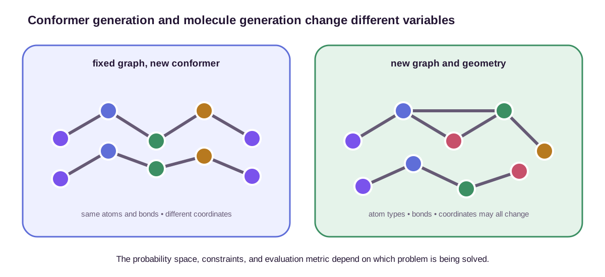
The distinction controls evaluation. Conformer methods are compared by ensemble coverage, precision, RMSD after alignment, energy distributions, and sometimes Boltzmann-weighted observables. Molecule generators are evaluated by chemical validity, uniqueness, novelty, graph–geometry consistency, stability after relaxation, and downstream property distributions. Mixing these metrics makes a model appear to solve a problem it was never asked to represent.

One graph, three populated conformers

Take n-butane as a deliberately small example. Its heavy-atom graph is fixed: four carbons in a chain. Rotation about the central carbon–carbon bond produces an anti basin near \(180^\circ\) and two symmetry-related gauche basins near \(+60^\circ\) and \(-60^\circ\). No atom identity or bond changes when the molecule moves between these basins. A graph generator would regard all three as the same output; a conformer generator must represent their distinct coordinates and populations.

To make the ensemble arithmetic explicit, use a two-energy approximation at \(T=298\,\mathrm{K}\). Set the anti free energy to zero and each gauche free energy to \(0.50\,\mathrm{kcal\,mol^{-1}}\). This is a toy thermodynamic model, not a claim that a single number captures solvent, vibrational, and force-field effects. Since

\[RT=(1.987\times10^{-3}\,\mathrm{kcal\,mol^{-1}\,K^{-1}})(298\,\mathrm{K}) \approx0.592\,\mathrm{kcal\,mol^{-1}},\]

each gauche state has relative weight

\[w_g=\exp\!\left(-\frac{0.50}{0.592}\right)\approx0.430.\]

The partition function for one anti and two gauche states is \(Z=1+2w_g=1.860\). Therefore

\[p_{\mathrm{anti}}=\frac{1}{Z}=0.538, \qquad p_{g^+}=p_{g^-}=\frac{0.430}{Z}=0.231.\]

The two gauche basins together hold \(46.2\%\) of the population even though neither is the minimum. Degeneracy competes with energy. A conformer method that always returns the anti geometry has perfect access to the lowest basin but misses nearly half of this simplified equilibrium ensemble.

Population errors propagate to observables. Suppose a hypothetical carbon-end-to-end distance is \(3.9\,\text{\AA}\) in anti and \(3.1\,\text{\AA}\) in either gauche state. The equilibrium average is

\[\langle d\rangle =0.538(3.9)+0.462(3.1) =3.53\,\text{\AA}.\]

Lowest-energy-only prediction gives \(3.90\,\text{\AA}\); giving the three basins equal weight gives \(3.37\,\text{\AA}\). Both enumerate chemically sensible conformers, yet both answer the ensemble question incorrectly. Coverage asks whether the basins were found. Calibration asks whether their mass was right. Those are separate requirements.

Three-dimensional probability lives modulo rigid motion

If \(\mathbf{Q}\in SO(3)\) and \(\mathbf{t}\in\mathbb{R}^3\), then

\[\mathbf{R}' =\mathbf{R}\mathbf{Q}^{\mathsf T} +\mathbf{1}\mathbf{t}^{\mathsf T}\]

describes the same isolated molecular geometry in a different laboratory frame. A physical density must assign equivalent probability to every such representation:

\[p(\mathbf{R}\mid G) =p(\mathbf{R}'\mid G).\]

Translation is often removed by centering the coordinates,

\[\widetilde{\mathbf{r}}_i =\mathbf{r}_i -\frac{1}{N}\sum_j\mathbf{r}_j.\]

Rotation remains as a symmetry. A Cartesian diffusion model can use an equivariant denoiser or score, so rotating the noisy molecule rotates the predicted coordinate update. EDM applies this idea while jointly denoising coordinates and categorical atom features (Hoogeboom et al., 2022). Permutations of indistinguishable atom labels introduce another symmetry that the graph architecture must respect.

The density is invariant, but the coordinate score is equivariant:

\[\nabla_{\mathbf{R}'}\log p(\mathbf{R}'\mid G) =\left(\nabla_{\mathbf{R}}\log p(\mathbf{R}\mid G)\right)\mathbf{Q}^{\mathsf T}.\]

This is not decorative data augmentation. It prevents the generator from spending capacity on arbitrary frame conventions and ensures that a rotated noisy state receives a correspondingly rotated denoising direction.

The same logic applies to continuous flows. A velocity field must be tangent to the centered coordinate subspace and equivariant under rotation. The geometric flow-matching post develops this construction for Euclidean, rotational, and product manifolds.

A centering and score check

The identities become less abstract on three points. Let

\[\mathbf r_1=(1,0,0),\quad \mathbf r_2=(0,2,0),\quad \mathbf r_3=(-1,0,0).\]

Their centroid is \((0,2/3,0)\), so the centered coordinates are

\[\widetilde{\mathbf r}_1=(1,-2/3,0),\quad \widetilde{\mathbf r}_2=(0,4/3,0),\quad \widetilde{\mathbf r}_3=(-1,-2/3,0),\]

which sum to zero. Translate every point by \(\mathbf t=(3,-1,2)\). The new centroid is the old centroid plus \(\mathbf t\), so subtracting it returns exactly the same three centered coordinates. Centering removes translation algebraically; it does not ask the model to learn translation invariance from examples.

For a concrete equivariant vector field, use the score of an isotropic centered Gaussian, \(\mathbf s_i=-\widetilde{\mathbf r}_i\). The three score vectors sum to zero, so an infinitesimal update stays in the centered subspace. Rotate by \(90^\circ\) around the \(z\) axis, \(Q(x,y,z)=(-y,x,z)\). The first centered point becomes \((2/3,1,0)\), and its new score is \((-2/3,-1,0)=Q(-1,2/3,0)\). The same equality holds atom by atom:

\[\mathbf s(Q\widetilde{\mathbf R})=Q\mathbf s(\widetilde{\mathbf R}).\]

This numerical check is modest but useful. In code, one can translate and rotate a noisy batch, run the network twice, undo the rotation on its second output, and compare the vectors. A large discrepancy diagnoses a broken equivariance contract before any sample-quality metric is computed. The manifold companion develops the corresponding transport geometry; here the point is operational: coordinate preprocessing, network outputs, and sampler updates must obey the same symmetry.

Cartesian and torsional models choose different state spaces

Cartesian generation perturbs every atomic coordinate. It is flexible: the model can change bond lengths, bond angles, torsions, and global shape. That flexibility makes the prior simple—usually centered Gaussian noise—but asks the network to relearn strong local chemical constraints. Independent coordinate noise readily creates distorted bonds and atomic clashes at intermediate times.

Internal-coordinate methods instead parameterize bond lengths, angles, and dihedral angles. For a fixed graph whose local geometry is supplied or separately generated, much conformational flexibility lies in \(m\) rotatable torsions,

\[\boldsymbol{\tau} =(\tau_1,\ldots,\tau_m) \in\mathbb{T}^m,\]

where each angle belongs to a circle and the full space is a torus. Torsional diffusion places its stochastic process on this periodic space and rotates whole molecular fragments about bonds (Jing et al., 2022). Bond lengths and most local angles remain fixed by construction.

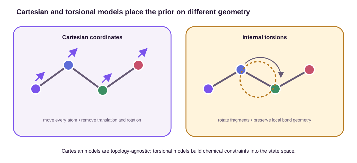
The restriction is both strength and limitation. Torsional generation is efficient for flexible organic molecules whose graph and local stereochemistry are known. It is less natural when rings change conformation, bonds form or break, coordination geometry varies, or local bond lengths respond strongly to environment. Cartesian methods are more general, but usually need stronger equivariant architectures, geometric regularization, or relaxation.

Latent 3D models add a second compromise. An encoder compresses graph and geometry into invariant and equivariant latent variables; diffusion or flow is performed in the smoother latent space; a decoder reconstructs the molecule. Sampling can be cheaper, but validity now depends on decoder coverage. A latent point that is numerically nearby need not decode to a chemically nearby structure.

Periodicity is a constraint, not a cosmetic encoding

Angles expose why the state space matters. The conformations at \(179^\circ\) and \(-179^\circ\) are only \(2^\circ\) apart on a circle, although direct subtraction gives \(-358^\circ\). The signed shortest displacement is

\[\Delta\tau =\operatorname{atan2}\!\left(\sin(\tau_2-\tau_1), \cos(\tau_2-\tau_1)\right) =2^\circ\]

for \(\tau_1=179^\circ\) and \(\tau_2=-179^\circ\). A Euclidean squared loss on raw degrees assigns error \(358^2=128{,}164\), whereas the periodic loss assigns \(2^2=4\). Encoding a torsion as \((\cos\tau,\sin\tau)\) or using a wrapped transition kernel prevents the branch cut from becoming a false barrier.

Internal coordinates also change what is held fixed. A torsional update can preserve a supplied bond length of \(1.54\,\text{\AA}\) and a bond angle of \(112^\circ\) exactly while rotating an entire downstream fragment. That is valuable when those quantities are trustworthy. It is restrictive when relaxation should shorten a conjugated bond, open a strained angle, or coordinate a ring closure. In an acyclic Z-matrix, a sequence of valid local lengths, angles, and torsions reconstructs coordinates. In a ring, locally valid entries need not make the final atoms meet: closure is a global constraint.

Cartesian coordinates reverse the bargain. Every coordinate array is a point configuration, and ring closure is represented directly by the positions of bonded atoms. But a Gaussian perturbation can turn a \(1.54\,\text{\AA}\) bond into \(0.7\,\text{\AA}\) or \(3.0\,\text{\AA}\) unless the learned field restores local chemistry. Cartesian validity is geometric existence, not chemical plausibility. Internal-coordinate validity preserves chosen local constraints, not necessarily global consistency. The right representation follows the deformations the application must permit.

Diffusion and flow learn a prior before optimization begins

A diffusion model defines a noising path from molecular data toward a simple reference distribution, then learns the reverse score or denoising field. A flow model learns a time-dependent velocity that transports the reference distribution toward data. In either case, the unconditional model represents a prior over plausible molecules:

\[p_\theta(x),\]

where \(x\) may be a conformer, a graph–coordinate pair, or a latent representation.

The prior matters during design. Direct optimization of a property predictor over unconstrained coordinates can create meaningless adversarial structures. Searching through a learned generator restricts proposals toward regions that resemble its training data. This is useful, but it is not a guarantee: a generator may reproduce dataset biases, miss rare but feasible chemistry, or assign probability to structures that pass representation-level validity while failing quantum relaxation.

Conditional generation changes the target to

\[p_\theta(x\mid c),\]

where \(c\) can be a desired property, a protein pocket, a scaffold, a fragment arrangement, or a symmetry constraint. Conditioning may be trained directly when paired data are available. Protein-specific 3D generators, for example, condition ligand placement and chemistry on a target pocket rather than optimizing a ligand in isolation.

When an unconditional score \(s_\theta(x,t)\) and a differentiable condition model \(p_\phi(c\mid x_t)\) are available, guidance uses

\[s_{\mathrm{guided}}(x_t,t) =s_\theta(x_t,t) +w\nabla_{x_t}\log p_\phi(c\mid x_t).\]

The first term follows the learned molecular prior; the second bends the reverse process toward the condition. Classifier-free guidance learns conditional and unconditional predictions in one model and combines them without an external gradient.

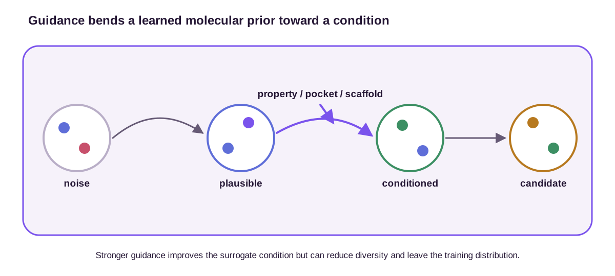
Increasing \(w\) usually improves the surrogate condition at the cost of diversity and distributional fidelity. More guidance is not universally better. If the condition model is least accurate off distribution, strong guidance drives sampling precisely where its gradients are least trustworthy.

Guidance tilts a finite prior

The prior–reward compromise is visible without a diffusion solver. Consider two molecular states. A familiar state \(A\) has prior mass \(p_0(A)=0.9\) and reward \(r(A)=0\). A rare state \(B\) has prior mass \(p_0(B)=0.1\) and reward \(r(B)=2\). An exponential tilt gives

\[p_\lambda(x) =\frac{p_0(x)e^{\lambda r(x)}} {\sum_{x'}p_0(x')e^{\lambda r(x')}}.\]

At \(\lambda=1\), the unnormalized masses are \(0.9\) and \(0.1e^2=0.739\), hence \(p_1(B)=0.451\). The higher-reward state still does not dominate because the learned prior regards it as rare. At \(\lambda=2\), its mass becomes \(0.1e^4=5.460\) and \(p_2(B)=0.858\). Guidance has not removed the prior; it has changed the relative leverage of prior density and reward. If \(r\) is an unreliable learned score on rare states, the second distribution is precisely the dangerous regime.

This finite example also clarifies why conditional success cannot be reported without diversity. Suppose three terminal objects have positive GFlowNet rewards \((1,4,9)\) and the target is \(p_T(x)\propto R(x)^{1/T}\). At \(T=1\) their probabilities are

\[(1,4,9)/14=(0.071,0.286,0.643).\]

At \(T=2\), taking square roots gives \((1,2,3)/6=(0.167,0.333,0.500)\). At \(T=0.5\), squaring gives \((1,16,81)/98=(0.010,0.163,0.827)\). Lower temperature increases selectivity but spends most samples on one mode; higher temperature preserves more alternatives at the price of lower mean reward. Neither temperature is intrinsically correct. A batch of twenty expensive assays may justify broader mass if oracle errors are correlated within a chemotype, while a reliable cheap oracle may justify concentration.

Goal-directed design is search under an imperfect oracle

Let \(R(x)\) be a computational oracle: a property predictor, docking score, quantum calculation, synthesis score, or weighted combination. Goal-directed design seeks candidates with large reward under a limited number of oracle evaluations.

Several strategies fit this template. A genetic algorithm mutates and recombines molecular representations. Reinforcement learning treats construction as a sequence of actions. Latent optimization encodes a molecule as \(z\), fits a surrogate \(\widehat R(z)\), searches continuous latent space, and decodes promising points. The continuous molecular representation of Gómez-Bombarelli et al. established this influential encoder–predictor–decoder pattern (Gómez-Bombarelli et al., 2018).

Latent optimization succeeds only where three maps remain aligned:

\[x\xrightarrow{\text{encode}}z, \qquad z\xrightarrow{\text{predict}}\widehat R, \qquad z\xrightarrow{\text{decode}}x'.\]

A large predicted reward is useless if the decoder is invalid or discontinuous there. Retraining on high-scoring samples can move the latent model toward the search distribution, but can also narrow diversity and amplify oracle artifacts.

GFlowNets pursue a different goal: sample diverse objects with probability proportional to a positive reward rather than collapse onto one maximizer (Bengio et al., 2021):

\[p(x)\propto R(x)^{1/T}.\]

The temperature \(T\) controls selectivity. This objective is attractive when many chemically distinct modes should be tested because the oracle is uncertain or batch experiments benefit from diversity. It still inherits the reward’s misspecification and the construction space’s limitations.

Oracle budget is a critical axis. An approach that finds a high score after one million predictor queries may be irrelevant when each query is a costly docking calculation or assay. The Practical Molecular Optimization benchmark shows that rankings can change substantially when algorithms share a fixed query budget (Gao et al., 2022). Reported results should therefore include the entire best-so-far curve, repeated seeds, and the number and cost of oracle evaluations—not only the best molecule found.

Multi-objective design is not one scalar in disguise

Real candidates must balance potency, selectivity, solubility, permeability, metabolic stability, toxicity, novelty, and synthesis cost. Writing

\[R(x)=\sum_{k=1}^K w_k R_k(x)\]

is convenient, but the weights encode a policy decision and can hide tradeoffs. A small change in normalization can reorder every candidate. Hard constraints such as forbidden substructures or maximum toxicity are not always well represented by a soft penalty.

The Pareto view is more transparent. Candidate \(x\) dominates \(y\) if it is no worse on every objective and better on at least one. The nondominated set exposes the frontier of tradeoffs rather than pretending that one weighting is uniquely correct. In practice, one can combine hard feasibility filters, calibrated uncertainty bounds, and Pareto ranking, then let downstream experiments or domain experts choose among diverse frontier candidates.

Three-dimensional objectives also depend on conformer choice. A docking score for one pose is not a molecular property independent of geometry. Fair evaluation may require generating multiple conformers, accounting for protonation and tautomer states, relaxing the complex, and aggregating across poses. Optimizing the easiest pose to score can exploit the docking pipeline rather than improve binding.

A frontier whose winner depends on policy

Consider three candidates scored on normalized potency, solubility, and synthetic convenience, all with larger values preferred:

candidate	potency	solubility	synthesis
P	9	3	8
Q	7	7	7
R	5	9	4

None dominates another. With weights \((0.6,0.2,0.2)\), their scalar utilities are \((7.6,7.0,5.6)\) and P wins. Equal weights give \((6.67,7.00,6.00)\) and Q wins. Solubility-heavy weights \((0.2,0.6,0.2)\) give \((5.2,7.0,7.2)\) and R wins. The optimizer did not discover three contradictory truths. It answered three different policy questions. Reporting only the winning scalar hides this dependence.

Now suppose P’s potency score of 9 came from its best docked conformer. It has two relevant conformer basins: a \(40\%\) state with pose score 10 and a \(60\%\) state with pose score 2. Under the simplifying assumption that these weights apply in the assay environment and that the score can be averaged linearly, its conformer-aware potency is

\[\bar R_{\mathrm{pot}}(P)=0.4(10)+0.6(2)=5.2.\]

The potency-heavy utility falls from \(7.6\) to

\[0.6(5.2)+0.2(3)+0.2(8)=5.32,\]

so Q at \(7.0\) becomes the winner. The assumptions are strong: binding can reweight conformers, docking scores need not be linear free energies, and protonation states add another ensemble. That is exactly why “optimize the best pose” is not an innocuous shortcut. A molecule-level objective needs a declared aggregation rule over the states available at inference and experiment.

Oracle exploitation is the default, not an edge case

Optimization induces distribution shift. A predictor trained on ordinary molecules is queried on candidates selected specifically to maximize its output. Even an unbiased in-distribution predictor becomes optimistically biased after selecting the top of a large pool, because positive errors are preferentially retained.

If

\[\widehat R(x)=R(x)+\epsilon(x),\]

then maximizing \(\widehat R\) selects both true reward and favorable error. The optimizer may exploit fingerprint shortcuts, docking clashes, unstable charge states, strained geometries, or regions where the uncertainty model is overconfident.

Several defenses work together:

• use ensembles or calibrated predictive distributions and penalize uncertainty;
• cap distance from the training domain or require similarity to validated chemistry;
• rescore finalists with an independent method that has different failure modes;
• adversarially audit repeated motifs and pathological geometries;
• reserve a hidden oracle or prospective evaluation that never guides optimization;
• optimize batches for diversity rather than near-duplicates around one apparent maximum.

Uncertainty is not a universal shield. Ensemble members sharing data and architecture can agree on the same wrong extrapolation. Domain checks, physical relaxation, and independent calculations remain necessary.

Maximization manufactures optimism

First isolate the statistical effect. Suppose \(N\) candidates have the same true reward \(\mu\), while oracle errors are independent \(\epsilon_i\sim\mathcal N(0,\sigma^2)\). The selected score is

\[\max_i\widehat R_i =\mu+\max_i\epsilon_i.\]

For a large pool, the leading extreme-value estimate is

\[\mathbb E[\max_i\epsilon_i] \approx \sigma\sqrt{2\log N}.\]

With \(N=10{,}000\) and \(\sigma=0.5\) reward units, this is

\[0.5\sqrt{2\log(10{,}000)} =0.5\sqrt{18.42} \approx2.15.\]

The formula is a leading approximation and slightly overstates the finite-normal maximum because it omits lower-order corrections. Its message is robust: a large proposal pool can produce a spectacular apparent gain even when every candidate is equally good. Increasing generation throughput without improving the oracle increases the opportunity to select error.

An independent rescore behaves differently. Let \(j=\arg\max_i(\mu+\epsilon_i)\) and evaluate the selected candidate with \(\widetilde R_j=\mu+\eta_j\), where \(\eta\) is independent of all selection errors and has mean zero. Conditional on the selection, \(\mathbb E[\eta_j]=0\), so \(\mathbb E[\widetilde R_j]=\mu\). The rescore does not make the molecule better; it removes the positive error that caused selection. In real design, the candidates have different true rewards and scoring methods share biases, so the correction is incomplete. Independence is a design goal, not an automatic property of running the same model twice.

A five-candidate query ledger

The small table below makes the decision visible. The primary oracle reports mean \(\mu\) and standard deviation \(\sigma\). “Independent” is a frozen higher-fidelity rescore unavailable during generation, and “measured” is a hypothetical eventual outcome.

candidate	primary \(\mu\)	\(\sigma\)	\(\mu-\sigma\)	independent rescore	measured reward
A	9.2	1.8	7.4	6.7	6.8
B	8.6	0.4	8.2	8.2	8.3
C	8.1	0.3	7.8	7.9	8.0
D	7.9	0.2	7.7	7.8	7.8
E	7.5	1.0	6.5	8.7	8.6

Raw maximization selects A, the noisiest candidate, and predicts 9.2; independent scoring drops it to 6.7. The conservative rule \(\mu-\sigma\) selects B and is rewarded here. But pure uncertainty penalization ranks E last even though it is the best measured candidate. Avoiding exploitation and exploring uncertain regions are competing purposes, not one formula with the sign changed.

That conflict is why a query budget should be declared before looking at results. Suppose the expensive measurement budget is five and the acquisition order is A (raw exploit), B (conservative exploit), E (uncertainty-bearing alternative), C, D. The measured best-so-far curve is

expensive queries used	selected candidate	measured reward	best so far
1	A	6.8	6.8
2	B	8.3	8.3
3	E	8.6	8.6
4	C	8.0	8.6
5	D	7.8	8.6

At budget one, the optimizer fails; at budget two, conservative selection looks best; at budget three, deliberate exploration wins. Quoting only the final 8.6 erases the cost and the acquisition decisions that produced it. A fair comparison freezes the candidate-generation allowance, every oracle query class, the batch size, and whether rescoring counts against the budget. It plots best measured reward against cumulative cost over repeated runs.

This ledger also separates three uncertainties often conflated in one error bar: uncertainty in the learned predictor, disagreement between computational fidelities, and experimental variation. A calibration curve for ordinary held-out molecules addresses only the first on that population. The selected tail needs its own prospective audit.

Synthesizability belongs inside the search loop

Representation-level validity asks whether a graph satisfies formal valence rules. Synthesizability asks whether available reagents and reactions provide a plausible route under practical constraints. These are far apart. Gao and Coley found that high-scoring generative proposals can be difficult for a synthesis planner to realize (Gao & Coley, 2020).

A heuristic synthetic-accessibility score is useful for filtering, but it is only a proxy. Stronger approaches generate through known fragments or reaction templates, query a retrosynthesis planner during optimization, or construct a sequence of reactions whose terminal product is the candidate. Reaction-constrained generation narrows chemical space, yet every generated object comes with at least one proposed route. The remaining questions—yield, selectivity, reagent availability, protection chemistry, and scale—still require evaluation.

The graph generation and reaction modeling chapter develops the mechanics of reaction edits, atom mapping, multistep search, route yields, and route-level denominators. The distinction matters here. A 3D optimizer may propose a stereochemically precise conformer because it scores well in a pocket; a synthesis planner operates on molecular identity and must find a route that produces the intended stereoisomer. A route to the correct connectivity but an unresolved racemate is not necessarily a route to the optimized object.

Synthesizability also interacts with diversity. A generator that repeatedly decorates one easy scaffold may score well on route success but offer little scientific breadth. Reports should distinguish graph diversity, scaffold diversity, three-dimensional shape diversity, and diversity among actually synthesizable candidates.

Experimental validation closes the epistemic loop

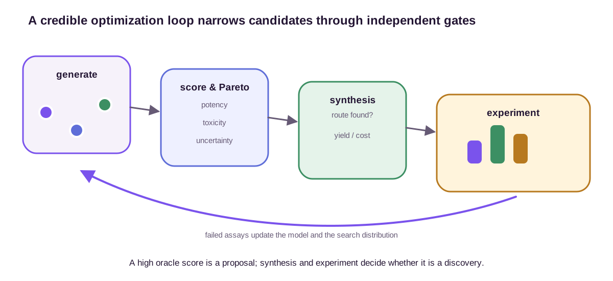
The computational endpoint should be a batch of hypotheses, not a declaration of discovery. Final candidates need structural sanitization, charge and stereochemistry assignment, conformer generation, quantum or force-field relaxation, independent rescoring, retrosynthetic review, and experimental prioritization. Each stage should record attrition rather than silently replace failed candidates.

Prospective validation is the decisive test because it prevents information leakage from benchmark construction. Synthesize a preregistered or otherwise frozen batch, measure the relevant endpoints with appropriate controls and replicates, and report success rate as well as the best success. Negative results reveal where the property model, generator, synthesis model, or assay assumptions were wrong.

A batch contract that can survive feedback

A credible closed loop can be stated before the first proposal:

1. Freeze the round. Version the generator, property models, conformer protocol, training set, admissible chemical space, and all thresholds. Declare an expensive-query budget—say 24 syntheses and assays—and a cheaper computational budget separately.
2. Generate and deduplicate. Produce the proposal pool once. Record failures before sanitization, then deduplicate by molecular identity, scaffold, stereochemistry, and the 3D diversity notion relevant to the task. Do not silently replace invalid outputs until the batch is full.
3. Score without feedback. Apply the frozen conformer ensemble, property oracles, domain checks, independent rescoring, and route planner. Keep every intermediate score and attrition reason. A candidate that lacks a route under the declared planner budget is a route-search failure, not proof of impossibility.
4. Choose a fixed batch. Reserve capacity for distinct purposes—for example, 12 conservative high-utility candidates, 6 Pareto-diverse alternatives, and 6 high-information candidates. Count close analogues explicitly so apparent sample size does not hide one repeated chemotype.
5. Attempt every candidate. Report how many entered synthesis, how many routes were attempted, which steps failed, how many compounds were obtained and confirmed, and how many yielded valid assay measurements. The denominator remains the original 24, not only the compounds that reached the plate.
6. Open the outcomes, then update. Only after the round closes may the measured results enter model fitting. Preserve the old model to evaluate calibration and ranking on the complete prospective batch. Define the next round using all outcomes, including synthesis and assay failures.

This contract creates several claim-matched endpoints. Distribution learning is supported by held-out likelihood or ensemble coverage, not by the best optimized molecule. Optimization is supported by best-so-far and hit-rate curves against query cost. Uncertainty is supported by calibration on selected candidates. Synthesis is supported by attempted-route success. Experimental utility is supported by the preregistered batch, controls, and replicates. No single aggregate score can substitute for all five.

Feedback then becomes scientifically useful rather than cosmetically iterative. If candidates pass computation but fail relaxation, the geometric prior or energy filter needs revision. If they relax but lack routes, the construction space and route objective are misaligned. If they are made but fail the assay, the property oracle or biological hypothesis is wrong. If one scaffold succeeds repeatedly, the next batch should decide whether to exploit it or test a counterfactual chemotype. Each failure localizes a different broken link.

The next iteration should learn from all tested compounds, including failures. Active discovery is a sequential decision problem: update predictive uncertainties, revise objective thresholds, and choose a new diverse batch with high value of information. The most useful molecule is not always the one with the highest predicted score; it may be the one that most clearly distinguishes competing hypotheses while remaining feasible to make.

Three-dimensional molecular generation gives us a geometrically legal way to propose structures. Conditional diffusion, flows, latent search, reinforcement learning, and GFlowNets give us different mechanisms for moving toward goals. None removes the central difficulty: optimization magnifies every weakness in the oracle and every omission in the representation. A credible design system therefore treats symmetry, chemical validity, diversity, uncertainty, synthesis, and experiment as one connected chain of evidence.

---

References

1. Hoogeboom, E., Garcia Satorras, V., Vignac, C., & Welling, M. (2022). Equivariant diffusion for molecule generation in 3D. Proceedings of the 39th International Conference on Machine Learning, 8867–8887. ↩
2. Jing, B., Corso, G., Chang, J., Barzilay, R., & Jaakkola, T. S. (2022). Torsional diffusion for molecular conformer generation. Advances in Neural Information Processing Systems, 35. ↩
3. Gómez-Bombarelli, R., Wei, J. N., Duvenaud, D., Hernández-Lobato, J. M., Sánchez-Lengeling, B., Sheberla, D., Aguilera-Iparraguirre, J., Hirzel, T. D., Adams, R. P., & Aspuru-Guzik, A. (2018). Automatic chemical design using a data-driven continuous representation of molecules. ACS Central Science, 4(2), 268–276. ↩
4. Bengio, E., Jain, M., Korablyov, M., Precup, D., & Bengio, Y. (2021). Flow network based generative models for non-iterative diverse candidate generation. Advances in Neural Information Processing Systems, 34. ↩
5. Gao, W., Fu, T., Sun, J., & Coley, C. W. (2022). Sample efficiency matters: A benchmark for practical molecular optimization. Advances in Neural Information Processing Systems, 35. ↩
6. Gao, W., & Coley, C. W. (2020). The synthesizability of molecules proposed by generative models. Journal of Chemical Information and Modeling, 60(12), 5714–5723. ↩

---

Figure provenance. All four mol3dopt_ diagrams are original SVG illustrations generated by scripts/generate_mol3dopt_figures.py. They synthesize standard geometric-generation identities and optimization safeguards described in the cited primary literature; no third-party artwork is reproduced.