How Drug Discovery Turns Biological Hypotheses into Molecules

Adapted from my 2025 Machine Learning for Molecules lectures. The article follows the evidence chain from a disease mechanism to a clinical intervention, showing where molecular machine learning helps and why a molecular prediction is not yet a drug-discovery result.

A drug begins as a claim about causality: changing some biological process will improve a disease. A molecule is one possible intervention on that process. Between the claim and a medicine lie several different questions. Is the proposed target causal in patients? Can it be modulated selectively? Can a compound reach the relevant tissue at a tolerable dose? Does changing the target produce clinical benefit?

These questions are coupled, but they are not interchangeable. Excellent binding to a noncausal target is useless. Potent inhibition in a biochemical assay can disappear in cells. A compound that works in cells can be metabolized before reaching the tissue. A drug that engages its target can fail because the disease has an escape route or because toxicity leaves no therapeutic window.

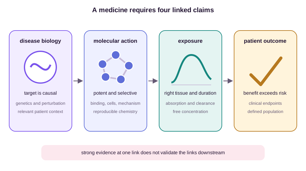
This is why drug discovery is better understood as a sequence of linked inference problems than as one molecular-optimization problem. Machine learning can reduce uncertainty at several links. It cannot turn a measurement at one link into evidence for all the others.

I will carry one hypothetical program through the chain. The program concerns a chronic inflammatory disease and a kinase called KX. Human genetics and patient-tissue data suggest that reducing KX signaling in inflammatory macrophages could lower disease activity. The team seeks a once-daily oral inhibitor. Its first credible chemical series contains compound A0; medicinal chemistry later selects A2. The names and numbers are illustrative, but every calculation uses ordinary quantities that a real program would have to connect: inhibition constants, association and dissociation rates, solubility, clearance, unbound tissue exposure, dose response, and randomized clinical outcomes.

The running example prevents a convenient fiction. No stage receives a fresh, ideal molecule. The affinity measured for A2 constrains the exposure it will need. Plasma binding changes how much of that exposure is pharmacologically available. The dose needed for target engagement changes the safety margin. The biomarker chosen in the clinic determines which failure explanations remain open.

The Starting Point Is a Biological Intervention

A target is a molecule or process whose modulation may alter disease: a receptor, enzyme, ion channel, protein–protein interaction, nucleic acid, or cellular phenotype. Target identification finds candidates. Target validation asks the harder counterfactual question:

If we intervene on this target in the relevant biological context, does the disease state improve?

Genetic association, perturbation experiments, disease models, human tissue, and prior pharmacology provide different kinds of evidence. Human genetics is especially valuable when allelic variation connects a target to both efficacy and safety phenotypes, but even then the molecular mechanism and therapeutically useful direction of modulation must be resolved (Plenge et al., 2013). A CRISPR knockout can reveal that a gene is necessary in a cell line, but complete deletion is not the same intervention as partial inhibition in an adult patient. An association can implicate a locus without identifying the causal gene. An animal model can reproduce one mechanism while missing human immune, metabolic, or developmental context.

The desired intervention must therefore be specified along with the target: inhibit or activate, continuously or transiently, in which tissue, cell type, disease stage, and patient population. The target alone is not the hypothesis.

Druggability is a separate question. A deep enzyme pocket may admit a conventional small molecule. A flat protein interface may require a macrocycle, peptide, degrader, antibody, or an indirect intervention. “Undruggable” often means that the current modality and assay do not provide enough control, not that biology forbids intervention.

Turning an association into an intervention claim

The KX program begins with three observations. A loss-of-function allele near the KX locus is associated with lower disease risk. KX expression is elevated in macrophages from active lesions. CRISPR interference lowers an inflammatory cytokine signature in patient-derived macrophages. The observations agree, but they answer different questions.

The genetic association concerns lifelong exposure to an allele across many tissues. The expression measurement is correlational: inflammation could raise KX rather than the reverse. CRISPR interference is an intervention, but it changes KX abundance for the duration and magnitude imposed by the experiment. An oral inhibitor instead changes catalytic activity according to its local free concentration. The drug hypothesis must bridge these interventions rather than treating them as synonyms.

Let \(Y(a)\) denote the disease outcome that would occur under intervention level \(a\), where \(a=1\) represents clinically achievable partial KX inhibition and \(a=0\) represents no inhibition. The causal quantity of interest is an average treatment effect in a defined patient population,

\[\tau=\mathbb{E}[Y(1)-Y(0)].\]

Neither high KX expression nor an accurate disease classifier identifies \(\tau\). The expression model estimates an association in observed data. Estimating the intervention effect requires randomization, a defensible natural experiment, or assumptions strong enough to reconstruct the counterfactual outcome. Human genetic evidence can strengthen the prior probability that KX is causal, but tissue, timing, and mechanism still differ from pharmacological inhibition.

The team therefore writes a narrower claim: sustained partial inhibition of KX catalytic activity in inflammatory macrophages will reduce the cytokine program in biomarker-positive adults without requiring KX inhibition in other tissues. This sentence determines the assay, desired direction, tissue exposure, biomarker, patient subgroup, and an early safety concern. “KX is the target” determines none of them.

The first experiments should separate the links. A biochemical assay asks whether a compound inhibits purified KX. A macrophage assay asks whether inhibition changes the proposed cytokine program. A rescue experiment with an inhibitor-resistant KX variant asks whether the cellular effect is on target. Measurements in hepatocytes and cardiomyocytes ask whether the same mechanism is hazardous elsewhere. A compound that changes the macrophage phenotype without engaging KX may still be interesting, but it no longer validates the proposed KX mechanism. The figure below shows the four claims that these experiments begin to connect.

Binding Is an Equilibrium, Not a Pose

For a simple reversible interaction

\[P+L \rightleftharpoons PL,\]

the dissociation constant is

\[K_d=\frac{[P][L]}{[PL]}, \qquad \Delta G^\circ=RT\log\frac{K_d}{C^\circ}.\]

Here \(C^\circ=1\) M is the standard concentration that makes the logarithm dimensionless.

A lower \(K_d\) means that less free ligand is needed to occupy the target at equilibrium. In the simplest one-site model, fractional occupancy is

\[\theta=\frac{[L]}{K_d+[L]}.\]

Occupancy follows from mass balance

The occupancy relation is worth deriving because it will later connect affinity to dose. Let \(P_{\mathrm{tot}}=[P]+[PL]\) be total target concentration and define \(\theta=[PL]/P_{\mathrm{tot}}\). Then \([PL]=\theta P_{\mathrm{tot}}\) and \([P]=(1-\theta)P_{\mathrm{tot}}\). Substituting these identities into the definition of \(K_d\) gives

\[K_d=\frac{(1-\theta)P_{\mathrm{tot}}[L]}{\theta P_{\mathrm{tot}}} =\frac{(1-\theta)[L]}{\theta}.\]

Solving for \(\theta\) yields the expression above. The cancellation of \(P_{\mathrm{tot}}\) assumes that \([L]\) denotes free ligand and that ligand depletion is negligible. If target concentration is comparable to the supplied ligand concentration, free ligand must be found from the full mass balance instead.

Suppose A2 has \(K_d=20\) nM. At a free concentration of 20 nM, occupancy is 50%. At 60 nM,

\[\theta=\frac{60}{20+60}=0.75.\]

Reaching 90% occupancy would require 180 nM, nine times the dissociation constant. Saturation creates diminishing returns: moving from 50% to 75% occupancy needs an additional 40 nM, while moving from 75% to 90% needs another 120 nM. The safety section will make the cost of that extra concentration explicit.

This equation exposes why a plausible docking pose is insufficient. A pose proposes geometry; affinity is a free-energy difference involving the bound and unbound ensembles, solvent, protonation, entropy, and competing states. A model can rank poses within one receptor structure and still miss affinity because the protein reorganizes, water is displaced, or the ligand adopts an expensive conformation.

Affinity is also not cellular potency. A biochemical assay may expose purified protein to a controlled free-ligand concentration. A cell adds membranes, transporters, metabolism, protein binding, target abundance, feedback, and off-targets. The half-maximal concentration reported by an assay—\(IC_{50}\) or \(EC_{50}\)—depends on the assay design and should not be silently interpreted as \(K_d\).

For a competitive enzyme inhibitor under the assumptions of Michaelis–Menten kinetics, the Cheng–Prusoff relation makes one source of protocol dependence explicit (Cheng & Prusoff, 1973):

\[K_i=\frac{IC_{50}}{1+[S]/K_m},\]

where \([S]\) is substrate concentration and \(K_m\) is the Michaelis constant measured under the same conditions. If the KX assay uses \([S]=4K_m\) and reports \(IC_{50}=100\) nM, then \(K_i=100/(1+4)=20\) nM. Running the assay at \([S]=K_m\) would instead produce \(IC_{50}=40\) nM for the same inhibitor. A model trained on the two values without protocol metadata sees label noise where enzymology sees a predictable shift.

Equal affinity can hide different clocks

Kinetics adds another dimension. The rates

\[k_{\mathrm{on}}[P][L] \quad\text{and}\quad k_{\mathrm{off}}[PL]\]

can yield the same \(K_d=k_{\mathrm{off}}/k_{\mathrm{on}}\) for compounds with different residence times. When exposure fluctuates, a slow off-rate may sustain target engagement after plasma concentration falls (Copeland et al., 2006). Whether this matters depends on target turnover and disease biology; residence time is not universally preferable.

Consider two inhibitors with the same \(K_d=20\) nM. A2 has

\[k_{\mathrm{on}}=5\times10^4\ \mathrm{M}^{-1}\mathrm{s}^{-1}, \qquad k_{\mathrm{off}}=10^{-3}\ \mathrm{s}^{-1},\]

while compound B has \(k_{\mathrm{on}}=5\times10^6\ \mathrm{M}^{-1}\mathrm{s}^{-1}\) and \(k_{\mathrm{off}}=10^{-1}\ \mathrm{s}^{-1}\). Both ratios are \(2\times10^{-8}\) M, yet their bound-state lifetimes differ by a factor of 100. For a first-order dissociation process after free ligand is removed,

\[[PL](t)=[PL](0)e^{-k_{\mathrm{off}}t}, \qquad t_{1/2,\mathrm{bound}}=\frac{\log 2}{k_{\mathrm{off}}}.\]

A2 has a mean residence time \(1/k_{\mathrm{off}}=1{,}000\) s and a bound-state half-life of 11.6 minutes. Compound B has a 10 s mean residence time and a 6.9 s half-life. Ten minutes after a washout, A2 retains \(e^{-0.001\times600}\approx55\%\) of its initially bound complexes. Compound B retains effectively none.

The slow off-rate helps only if persistent KX inhibition is desirable. If a transient pulse is safer, or if KX is rapidly resynthesized, the kinetic advantage can vanish. Association can also become too slow to track a short exposure. Affinity, association, dissociation, target turnover, and concentration–time history jointly determine engagement.

A Hit Is Evidence, Not a Starting Drug

Hit identification can use high-throughput screening, fragments, phenotypic screening, virtual screening, or prior chemical matter. A credible hit survives orthogonal confirmation and controls for aggregation, fluorescence interference, covalent reactivity, assay artifacts, and sample identity. Its structure and activity should be reproducible.

The next task is to establish a structure–activity relationship (SAR). Chemists make controlled changes and observe how potency, selectivity, solubility, permeability, metabolic stability, and toxicity respond. If large structural changes leave the signal unchanged, the assay may be reporting an artifact. If nearby analogues move activity smoothly, the series offers a path for optimization.

A small SAR table changes the question

The first KX series varies one solvent-exposed substituent while keeping the binding core fixed. Four representative analogues give the following profile. Intrinsic clearance, \(CL_{\mathrm{int}}\), is an in-vitro measure of metabolic turnover; lower is better. Off-target IC\(_{50}\) is measured against a related kinase whose inhibition is undesirable.

Compound	KX IC\(_{50}\) (nM)	Solubility (µM)	\(CL_{\mathrm{int}}\) (µL/min/mg)	Off-target IC\(_{50}\) (nM)
A0	250	140	18	15,000
A1	30	8	70	900
A2	100	65	20	8,000
A3	150	160	14	1,500

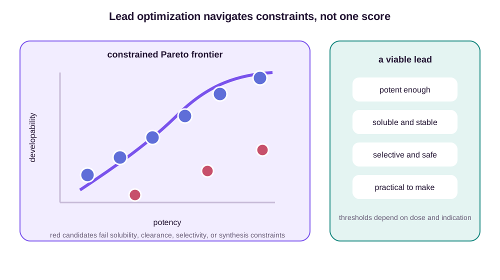
A1 is the most potent compound, but it is poorly soluble, rapidly metabolized, and only 30-fold selective by the ratio \(900/30\). A3 is soluble and stable but only tenfold selective. A0 has the widest selectivity ratio and acceptable developability, yet misses the potency goal. A2 is not best in any single column. It is the only analogue satisfying the program’s initial gates: KX IC\(_{50}\leq150\) nM, solubility at least 50 µM, \(CL_{\mathrm{int}}\leq30\) µL/min/mg, and off-target IC\(_{50}\geq5{,}000\) nM.

The table is a minimal SAR because nearby chemical changes move multiple measurements in interpretable ways. The substituent that improves potency in A1 also raises lipophilicity, lowering solubility and increasing metabolic turnover. That hypothesis can be tested with another matched pair. A model that proposes A1 because it has the best predicted potency has not solved the decision the chemist faces.

Suppose a lead must achieve target potency \(p(x)\), aqueous solubility \(s(x)\), microsomal stability \(m(x)\), and low off-target activity \(o(x)\). There is generally no molecule maximizing all four. A scalar score

\[J(x)=w_p p(x)+w_s s(x)+w_m m(x)-w_o o(x)\]

hides the choice of weights and can reward an unacceptable tradeoff. Medicinal chemistry instead navigates a Pareto frontier while enforcing hard constraints such as chemical stability, synthetic accessibility, and reactive-group exclusions.

For objective vector \(\mathbf{f}(x)\), compound \(x\) dominates compound \(x'\) if it is at least as good on every objective and strictly better on one. The Pareto set contains candidates that no other measured candidate dominates. A1 and A2 can both lie on that set: A1 trades developability for potency, while A2 gives up potency for a balanced profile. Pareto membership does not make A1 acceptable because hard constraints still apply.

A scalar score can reverse the choice without any new evidence. Converting 30 nM and 100 nM to \(pIC_{50}=-\log_{10}(IC_{50}\text{ in M})\) gives 7.52 for A1 and 7.00 for A2. If potency receives enough weight, the 0.52-log advantage can overwhelm normalized penalties for solubility and clearance. Raising the penalty weights makes A2 win. The ranking has changed because preferences changed, not because the molecules changed. The figure below separates the nondominated frontier from the hard developability gates.

This is where property-prediction and generative models are useful. A model can prioritize compounds, estimate uncertainty, propose analogues, and decide which assay would be informative next. But the training labels inherit protocol differences, censoring, batch effects, and series bias. Random molecular splits often place close analogues on both sides of evaluation, measuring interpolation within known chemistry rather than prospective discovery; benchmark studies have shown how readily such similarity turns memorization into apparent generalization (Wallach & Heifets, 2018). The broader issues of representation, conformers, splits, and uncertainty are developed in Molecular Data and Property Prediction.

For the KX program, the next useful prediction is not “which virtual compound has maximal potency?” It is “which analogue is most likely to clear all four gates, and which measurement would most change that probability?” A prospective test should count the denominator: among compounds the model selected for synthesis, how many were made, yielded valid measurements, and cleared the joint profile? Reporting only the potency of the best successful molecule erases synthesis failures and the compounds that violated another gate.

Exposure Connects a Molecule to a Tissue

Pharmacokinetics describes what the body does to a compound: absorption, distribution, metabolism, and excretion. After an oral dose, concentration often rises as the drug is absorbed, reaches a maximum \(C_{\max}\), then falls through distribution and clearance. The area under the concentration–time curve (AUC) measures total systemic exposure.

For a simple one-compartment intravenous model,

\[C(t)=C_0e^{-k_e t}, \qquad t_{1/2}=\frac{\log 2}{k_e}, \qquad CL=k_eV_d,\]

where \(CL\) is clearance and \(V_d\) is apparent volume of distribution. Real compounds may require multiple compartments, saturable processes, active transport, or time-varying metabolism, but the simple model makes one point clear: potency has meaning only relative to free concentration at the site of action.

Deriving an oral concentration curve

The KX inhibitor is intended for oral dosing, so absorption must enter the model. Let \(D\) be the dose, \(F\) the fraction reaching systemic circulation, \(k_a\) the first-order absorption rate, and \(k_e=CL/V_d\) the elimination rate. The amount entering plasma per unit time is \(FDk_ae^{-k_at}\). Mass balance in a one-compartment model gives

\[V_d\frac{dC}{dt}=FDk_ae^{-k_at}-CL\,C.\]

Dividing by \(V_d\) and multiplying by the integrating factor \(e^{k_et}\) yields

\[\frac{d}{dt}\left(e^{k_et}C(t)\right) =\frac{FDk_a}{V_d}e^{(k_e-k_a)t}.\]

Integrating from 0 to \(t\) with \(C(0)=0\) produces the Bateman function

\[C(t)=\frac{FDk_a}{V_d(k_a-k_e)} \left(e^{-k_et}-e^{-k_at}\right), \qquad k_a\neq k_e.\]

The two exponentials have different jobs. The absorption term initially cancels the elimination term, so concentration starts at zero. Once absorption is nearly complete, \(e^{-k_at}\) vanishes and the terminal slope is controlled by \(k_e\). Setting the derivative to zero gives the peak time

\[t_{\max}=\frac{\log(k_a/k_e)}{k_a-k_e},\]

while integrating concentration over time gives

\[AUC_{0\rightarrow\infty}=\frac{FD}{CL}.\]

The AUC identity shows why distribution volume changes the shape of the curve but not total exposure in this linear model. It is also an assumption boundary: dose-dependent clearance or bioavailability breaks the proportionality.

For A2, suppose early human predictions give \(D=200\) mg, \(F=0.50\), \(V_d=40\) L, \(CL=4\) L/h, and \(k_a=1.0\) h\(^{-1}\). Then \(k_e=0.10\) h\(^{-1}\), the elimination half-life is 6.93 h, and

\[t_{\max}=\frac{\log(1/0.1)}{1-0.1}=2.56\ \mathrm{h}.\]

Substituting this time into the concentration curve gives \(C_{\max}=1.94\) mg/L, while \(AUC=25\) mg·h/L. If A2 has molecular weight 500 g/mol, then 1 mg/L equals 2 µM, so the total peak plasma concentration is 3.87 µM.

Total plasma concentration can be misleading when most compound is bound to plasma proteins. Brain targets add the blood–brain barrier and efflux transporters. Intracellular targets add membrane permeability and sequestration. Prodrugs deliberately separate the administered molecule from the active species. Metabolites may be inactive, active, or toxic.

Free concentration is the bridge to occupancy

Let \(f_{u,p}\) be the unbound fraction in plasma and let \(K_{p,uu}\) be the ratio of unbound concentration at the site of action to unbound plasma concentration. Under a rapid-equilibrium approximation,

\[C_{u,\mathrm{site}}(t)=K_{p,uu}f_{u,p}C_{\mathrm{total},p}(t).\]

For A2, take \(f_{u,p}=0.02\) and \(K_{p,uu}=0.50\). The predicted free concentration in macrophage tissue at the total plasma peak is not 3.87 µM but

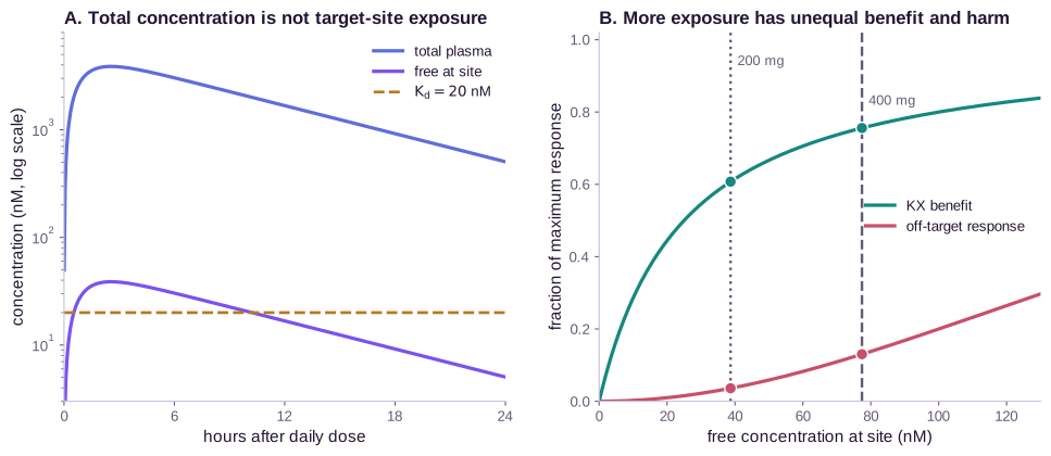
\[C_{u,\mathrm{site},\max} =0.50\times0.02\times3.87\ \mu\mathrm{M} =38.7\ \mathrm{nM}.\]

With \(K_d=20\) nM, the equilibrium occupancy estimate is \(38.7/(20+38.7)=66\%\). Comparing total plasma concentration directly with \(K_d\) would predict more than 99% occupancy and would be wrong by construction. Unbound concentration is the relevant comparison when passive distribution and rapid binding equilibrium are reasonable; active transport, lysosomal trapping, slow tissue exchange, and local metabolism require a richer model (Summerfield et al., 2022).

Peak occupancy is not duration. For a 24 h dosing interval, the linear repeated-dose model sums residual concentrations from all earlier doses. Just before the next dose,

\[C_{\mathrm{trough,ss}}= \frac{FDk_a}{V_d(k_a-k_e)} \left[ \frac{e^{-k_e\tau}}{1-e^{-k_e\tau}} -\frac{e^{-k_a\tau}}{1-e^{-k_a\tau}} \right],\]

where \(\tau=24\) h. The predicted steady-state trough is 0.277 mg/L total plasma, or 5.54 nM free at the site. Equilibrium occupancy would fall to 22%. A2’s 11.6 min bound-state half-life cannot bridge a 24 h trough. The team must therefore test whether transient daily inhibition is biologically sufficient, change dosing frequency or formulation, reduce clearance, or improve affinity without losing the balanced SAR profile.

Pharmacodynamics describes what exposure does to the biological system. A common saturating response model is

\[E(C)=E_0+\frac{E_{\max}C^h}{EC_{50}^h+C^h},\]

with Hill coefficient \(h\). The response may lag concentration because target turnover and downstream signaling have their own timescales. Biomarkers are valuable when they show that a dose reaches the tissue and engages the intended mechanism, rather than merely producing a correlated change.

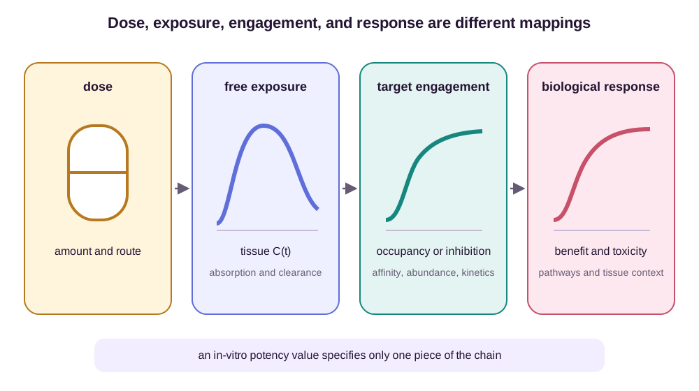
Exposure, engagement, and response can separate in time

Suppose KX engagement reduces the cytokine signal with \(EC_{50}=25\) nM, \(h=1\), and a maximum reduction of 80 percentage points. Ignoring delay, the predicted reduction at the 38.7 nM free peak is

\[\Delta E_{\max}=80\times\frac{38.7}{25+38.7}=48.6\]

percentage points. At the 5.54 nM trough, it is 14.5 points. These are model outputs conditional on the assumed tissue concentration and response parameters, not new measurements.

If cytokine messenger RNA decays slowly, the response can remain suppressed after occupancy falls. A simple effect-compartment model represents that lag by a latent concentration \(C_e\),

\[\frac{dC_e}{dt}=k_{e0}\left(C_{u,\mathrm{site}}-C_e\right),\]

where \(k_{e0}\) controls equilibration between measured exposure and observed effect. This differential equation does not identify the biological mechanism; it summarizes delay. Measuring both target engagement and the downstream cytokine marker is what distinguishes slow molecular dissociation from slow pathway recovery.

The figure below keeps the four mappings separate: administered dose, free tissue exposure, target engagement, and biological response.

Safety Is a Margin, Not a Binary Property

Any pharmacologically active molecule perturbs biology. The practical question is whether desired effects occur at exposures below those causing unacceptable harm. A schematic therapeutic index compares toxic and effective doses,

\[TI=\frac{TD_{50}}{ED_{50}},\]

but a single ratio suppresses the shape of both dose–response curves, patient variability, treatment duration, and severity of the adverse event.

A therapeutic-window calculation

For the running example, let desired KX benefit follow

\[B(C)=\frac{C}{25+C},\]

and let a safety-relevant off-target response follow a steeper curve

\[H(C)=\frac{C^2}{200^2+C^2},\]

where \(C\) is free concentration in nM and each function is scaled to its own maximum. These curves are illustrative. They make the dose tradeoff visible without pretending that efficacy and toxicity share one biological endpoint.

At the predicted 200 mg peak of 38.7 nM, \(B=0.61\) and \(H=0.036\). If linear pharmacokinetics holds, doubling the dose doubles concentration to 77.4 nM. Benefit rises to 0.76, but the off-target response rises to 0.13. A twofold dose increase buys 15 percentage points of normalized benefit while adding about 9 percentage points of normalized harm. Saturation, not a failure of optimization, creates this asymmetry.

We can also compare exposure thresholds. The concentration giving 50% benefit is 25 nM. Solving \(H(C)=0.10\) gives

\[C_{H=0.10}=200\sqrt{\frac{0.10}{0.90}}=66.7\ \mathrm{nM}.\]

The exposure margin from half-maximal benefit to 10% off-target response is only \(66.7/25=2.67\). Relative to the predicted 38.7 nM peak, the remaining margin is 1.72-fold. That margin must absorb errors in clearance, protein binding, tissue partition, off-target potency, and patient susceptibility.

Interpatient variability turns one curve into a distribution. If a patient clears A2 at 2 L/h rather than 4 L/h while other linear-model parameters remain similar, AUC doubles. Peak concentration will not necessarily double because absorption and distribution also shape it, but sustained exposure will rise. A dose selected from population-average PK can therefore cross the safety threshold in slow-clearance patients and miss the efficacy threshold in fast-clearance patients. Dose adjustment, exclusion criteria, or exposure monitoring are parts of the therapeutic window, not administrative details after molecular design.

The two scales in the calculation are easier to compare directly in the figure below. The left panel shows why total plasma exposure can remain orders of magnitude above \(K_d\) while free target-site concentration crosses below it; the right panel shows the benefit and off-target responses at the 200 mg and doubled-dose peaks.

Safety failures arise through several routes. On-target toxicity occurs when the intended mechanism is harmful in another tissue or at excessive inhibition. Off-target toxicity comes from unintended molecular interactions. Reactive metabolites, immune responses, organ accumulation, and drug–drug interactions add mechanisms that may not appear in an acute cellular assay.

Selectivity must therefore be evaluated against a relevant panel, not defined as “stronger binding to the intended target.” A tenfold affinity margin can disappear when the off-target is more abundant, the free tissue concentration differs, or its physiological response is steeper. Chronic dosing can expose liabilities invisible in a short experiment.

The relevant selectivity margin is exposure based. A2’s 80-fold biochemical selectivity ratio against the related kinase is reassuring, but it does not equal an 80-fold clinical window. The off-target may be expressed in a different tissue, bind A2 with another free fraction, or trigger harm at low fractional occupancy. Conversely, partial KX inhibition may be enough for benefit. The PK/PD and toxicity curves, not the affinity ratio alone, determine the usable dose range.

Machine-learning toxicity alerts are triage tools. They are strongest inside chemical and assay regimes represented in training and weakest for rare mechanisms, unusual metabolites, and new modalities—the very regions in which confident extrapolation is most dangerous.

Clinical Trials Test the Whole Causal Chain

Preclinical studies support a first human dose, but clinical development asks successively broader questions. Phase I emphasizes safety, tolerability, exposure, and often target engagement. Phase II asks whether the intervention shows efficacy in an appropriate patient population and refines dose. Phase III tests benefit and risk at the scale and rigor needed for registration. The boundaries vary by disease and modality, but the evidentiary progression remains.

Clinical failure is not one event. A trial may fail because the target was not causal, the drug did not reach or engage it, the dose was limited by toxicity, the endpoint was insensitive, the population was heterogeneous, or the trial was underpowered. Without exposure and engagement biomarkers, a negative efficacy result cannot distinguish a failed biological hypothesis from a failed intervention.

A biomarker ladder keeps denominators visible

The KX program defines four measurements before its early patient study:

1. Exposure: did unbound A2 concentration exceed the prespecified threshold?
2. Engagement: was KX occupancy or pathway-proximal inhibition observed?
3. Pharmacodynamic response: did the macrophage cytokine signature fall?
4. Clinical response: did the patient endpoint improve?

Suppose 30 patients receive 200 mg. Twenty-seven exceed the exposure threshold. Of those 27, twenty-two show target engagement. Of those 22, seventeen show the cytokine response. The conditional rates are 90%, 81%, and 77%, respectively. The unconditional fraction completing all three links is \(17/30=57\%\).

The denominator changes the claim. Reporting 17 of 22 makes A2 look like a reliable pathway modulator once exposure and engagement have already succeeded. Reporting 17 of 30 describes the probability that assigning the dose to a patient completes the chain. Both are correct, but they answer different decisions. Dose selection needs the second. Mechanistic diagnosis also needs the conditional transitions.

The failure branches are informative. Three patients failed at exposure, pointing to absorption, clearance, adherence, or measurement. Five had exposure without engagement, pointing to tissue partition, target abundance, affinity, or an incorrect engagement assay. Five had engagement without the cytokine change, weakening the proposed pathway link or exposing biological heterogeneity. Pooling all thirteen as “biomarker negative” destroys this structure.

The cytokine signature is a pharmacodynamic biomarker, not automatically a surrogate clinical endpoint. A valid surrogate must support inference about the treatment effect on the clinical outcome, a much stronger requirement than correlation with prognosis or response (Prentice, 1989). KX engagement can confirm that the intervention reached its molecular target without proving that patients will benefit.

A small randomized trial can support mechanism before efficacy is settled

Now suppose a randomized Phase II study assigns 30 patients to A2 and 30 to placebo. Fifteen treated patients and nine controls meet the clinical-response endpoint. The estimated response rates are

\[\hat p_T=\frac{15}{30}=0.50, \qquad \hat p_C=\frac{9}{30}=0.30,\]

so the estimated risk difference is 0.20. Under an independent-binomial approximation, its standard error is

\[SE(\hat p_T-\hat p_C)= \sqrt{\frac{0.50(0.50)}{30}+\frac{0.30(0.70)}{30}} =0.124.\]

A normal 95% confidence interval is \(0.20\pm1.96(0.124)=[-0.04,0.44]\). The point estimate is promising, but the interval includes no benefit. A Bayesian calculation with independent uniform priors gives posteriors \(p_T\mid\text{data}\sim\operatorname{Beta}(16,16)\) and \(p_C\mid\text{data}\sim\operatorname{Beta}(10,22)\). Numerical integration gives about 94% posterior probability that \(p_T>p_C\), while the 95% credible interval for the difference remains roughly \([-0.05,0.41]\). Neither framework turns 60 patients into a precise effect estimate.

The mechanistic measurements still change interpretation. If most treated patients reached the exposure and engagement thresholds and the cytokine signature moved in the predicted direction, the study establishes that A2 delivered the intended intervention. A weak clinical signal then focuses attention on target causality, disease stage, endpoint sensitivity, or population heterogeneity. If engagement failed, the same clinical result says little about KX biology.

Biomarker enrichment requires an interaction, not a favorable subgroup

Assume the macrophage signature was prespecified as a patient-selection biomarker. Among 20 biomarker-positive patients per arm, 13 respond to A2 and 6 to placebo: a risk difference of 0.35 with an approximate 95% interval of \([0.06,0.64]\). Among 10 biomarker-negative patients per arm, 2 respond to A2 and 3 to placebo: a difference of \(-0.10\) with interval \([-0.48,0.28]\).

It is tempting to call the biomarker predictive because one subgroup is statistically positive and the other is not. The relevant comparison is the interaction: does the treatment effect differ between subgroups? The estimated interaction on the risk-difference scale is \(0.35-(-0.10)=0.45\). Combining the two subgroup variances gives standard error 0.243 and an approximate 95% interval \([-0.03,0.93]\). The trial suggests enrichment but does not estimate the interaction precisely.

This distinction blocks a common retrospective story. Selecting the subgroup with the largest observed response and then reporting its within-group result uses the same noise twice. A confirmatory enrichment claim needs a prespecified rule or independent validation. Machine learning can construct a multivariate biomarker, but its evaluation unit is the randomized treatment-effect difference in the intended population, not its accuracy at predicting who happened to respond on treatment.

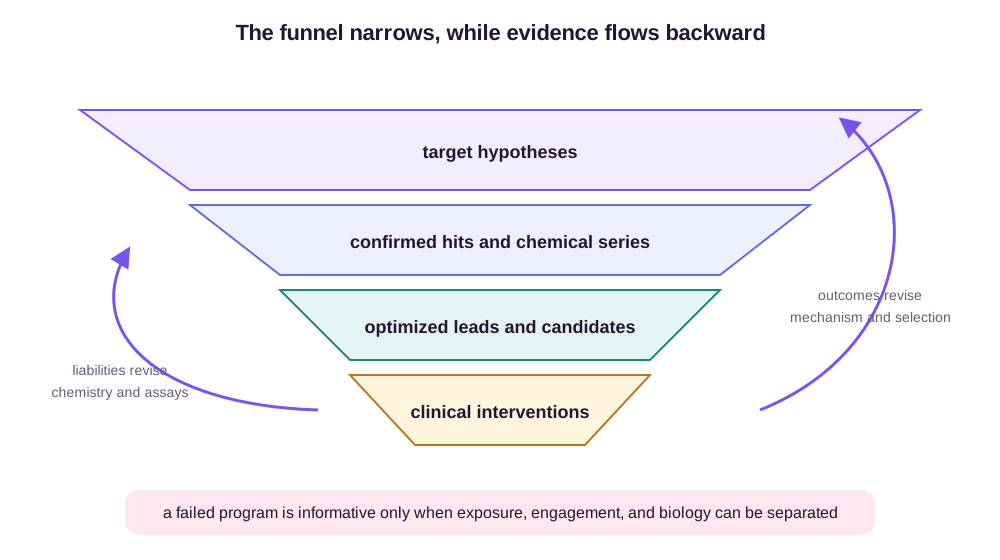
Published analyses show that transition probabilities vary strongly by therapeutic area and development phase, making overall “success rate” a property of a defined portfolio and time window rather than a universal constant (Wong et al., 2019). The long decline in output per inflation-adjusted research investment—often called Eroom’s law—also warns that adding more screening and computation does not automatically remove biological uncertainty (Scannell et al., 2012). The feedback paths in the next figure show why a late outcome must be assigned to a failed link before it can improve the next program.

Machine Learning Must Be Attached to a Decision

Drug-discovery data are generated by decisions. Chemists synthesize compounds they expect to work. Assays are run on selected series. Negative results may be censored or absent. Clinical candidates are an extreme, nonrandom subset of discovered molecules. A model trained on this record learns the selection process alongside chemistry.

This creates three common overclaims:

• Retrospective prediction becomes prospective value. A random split measures recognition of familiar series, not whether the model changes which compound should be made next.
• A surrogate becomes the objective. Generated molecules exploit a learned potency or synthesizability score outside its reliable region.
• A molecular endpoint becomes a program outcome. Better docking, affinity, or ADMET prediction is reported as faster drug discovery without tracing the downstream decision.

A useful evaluation starts from the decision. Did prioritization recover active compounds under a time or scaffold split? Did uncertainty identify measurements that improved the series? Did proposed compounds synthesize and reproduce their predicted profile? Did the model reduce experiments, calendar time, or failure risk compared with the actual alternative?

Evaluate the selected batch, including its failures

Suppose a model ranks 10,000 virtual KX analogues and selects 100 for synthesis. Seventy-two are successfully made, 65 yield valid measurements in every required assay, and 8 clear the joint potency, solubility, clearance, and selectivity profile. An expert-designed comparison batch of 100 yields 80 synthesized compounds, 70 complete profiles, and 5 joint successes.

Several rates can be reported:

Denominator	Model-selected batch	Expert batch
Assigned designs	8/100 = 8.0%	5/100 = 5.0%
Synthesized compounds	8/72 = 11.1%	5/80 = 6.3%
Complete assay profiles	8/65 = 12.3%	5/70 = 7.1%

The assigned-design denominator best matches the decision “which 100 proposals should consume the synthesis budget?” The complete-profile denominator isolates molecular profile quality after synthesis and assay attrition. Reporting only 8 versus 5 successful molecules is insufficient if the batches differ in cost, novelty, or time. Reporting only the best potency is worse because the program selected A2 for its joint profile.

An uncertainty model should also be judged by an action. If A4 has uncertain clearance and A5 has uncertain selectivity, which measurement is expected to change the next synthesis choice? A generic calibration curve does not answer that question. A useful acquisition rule values the expected change in program utility after observing assay \(y\),

\[a(x,\text{assay})= \mathbb{E}_{y\mid x,\mathcal{D}} \left[U(\mathcal{D}\cup\{(x,y)\})-U(\mathcal{D})\right] -\lambda\,\mathrm{cost}(x,\text{assay}),\]

where \(\mathcal{D}\) is current evidence and \(U\) represents the downstream decision. This is a design principle, not a claim that the exact utility is known. It forces the modeler to state what information is valuable and which cost is being saved.

Prospective, blinded tests are unusually valuable because they include the selection step. So are negative results: they reveal the model’s applicability boundary and improve the next acquisition round. The central unit is not a benchmark score but a closed experimental loop.

A Drug Is a Chain of Evidence

The discovery pipeline is often drawn as target identification, hit finding, hit-to-lead, lead optimization, preclinical development, and clinical trials. The drawing looks linear; the work is not. Poor cellular translation sends a team back to mechanism or permeability. Toxicity motivates new chemistry or a different modality. Patient biomarkers revise the target hypothesis. Every stage changes the distribution of questions at the next stage.

The most durable view is therefore a chain of claims:

1. intervening on a target changes relevant disease biology;
2. a molecule produces the intended intervention selectively;
3. a feasible dose creates sufficient exposure and engagement;
4. the intervention improves patient outcomes with acceptable risk.

Molecular machine learning operates mainly in the middle of this chain, where representations, property models, docking, simulation, and generation can make experimentation more selective. Its contribution becomes scientifically legible when it states which uncertainty is reduced and which claim remains untested.

The KX example now has one traceable chain. Genetics and perturbation motivate partial macrophage KX inhibition. Binding experiments identify A2’s affinity and kinetic timescale. SAR selects A2 because it clears a joint profile rather than maximizing potency. Oral PK predicts 38.7 nM peak free tissue concentration and 66% peak occupancy, but only 5.54 nM at the daily trough. The therapeutic calculation shows why doubling dose yields modest additional benefit and a larger off-target response. Clinical exposure, engagement, cytokine, and outcome measurements then determine whether a negative result challenges delivery, mechanism, population selection, or the target itself.

That boundary is not a limitation to hide. It is how a computational result becomes useful to a drug-discovery program.

---

References

Wong, C. H., Siah, K. W., & Lo, A. W. (2019). Estimation of Clinical Trial Success Rates and Related Parameters. Biostatistics, 20(2), 273–286. ↩

Scannell, J. W., Blanckley, A., Boldon, H., & Warrington, B. (2012). Diagnosing the Decline in Pharmaceutical R&D Efficiency. Nature Reviews Drug Discovery, 11, 191–200. ↩

Plenge, R. M., Scolnick, E. M., & Altshuler, D. (2013). Validating Therapeutic Targets through Human Genetics. Nature Reviews Drug Discovery, 12, 581–594. ↩

Copeland, R. A., Pompliano, D. L., & Meek, T. D. (2006). Drug–Target Residence Time and Its Implications for Lead Optimization. Nature Reviews Drug Discovery, 5, 730–739. ↩

Wallach, I., & Heifets, A. (2018). Most Ligand-Based Classification Benchmarks Reward Memorization Rather than Generalization. Journal of Chemical Information and Modeling, 58(5), 916–932. ↩

Cheng, Y., & Prusoff, W. H. (1973). Relationship Between the Inhibition Constant and the Concentration of Inhibitor Which Causes 50 Percent Inhibition of an Enzymatic Reaction. Biochemical Pharmacology, 22(23), 3099–3108. ↩

Summerfield, S. G., Yates, J. W. T., & Fairman, D. A. (2022). Free Drug Theory—No Longer Just a Hypothesis?. Pharmaceutical Research, 39, 213–222. ↩

Prentice, R. L. (1989). Surrogate Endpoints in Clinical Trials: Definition and Operational Criteria. Statistics in Medicine, 8(4), 431–440. ↩

---

Figure provenance. All five drugdisc_ figures are original SVG-first illustrations and plots generated by scripts/generate_drugdisc_figures.py. They synthesize standard pharmacological and drug-development concepts or render the illustrative calculations derived in the post; no lecture-slide, paper, or third-party icon artwork is reproduced.