On this page
Adapted from my 2025 Geometric Deep Learning lectures. The central question is how an infinite periodic solid becomes a finite, symmetry-aware object that can be predicted, generated, relaxed, and validated.
A Crystal Is Infinite, but Its Description Should Not Be
A molecule is usually represented as a finite collection of atoms. A perfect crystal repeats without end. That single difference changes the representation, the symmetry, and the meaning of generation.
Choose a lattice matrix
\[L=[\ell_1,\ell_2,\ell_3]\in\mathbb R^{3\times 3},\]whose columns are lattice vectors, and fractional coordinates \(s_i\in[0,1)^3\) for the atoms in one unit cell. The Cartesian coordinate is \(x_i=Ls_i\). The infinite set of images is
\[\mathcal C=\{(z_i,L(s_i+n)):i=1,\ldots,N,\ n\in\mathbb Z^3\},\]where \(z_i\) is the chemical element. The finite tuple \((A,L,S)\)—element types, lattice, and fractional sites—describes the infinite solid.
This description is not unique. Replacing \(s_i\) by \(s_i+n\) changes no atom. Reordering sites changes no material. A rigid rotation \(Q\) sends \(L\mapsto QL\) and every Cartesian position to \(Qx_i\) without changing a scalar property. Different choices of primitive or conventional cell can represent the same crystal. Space-group operations add rotations, reflections, screws, glides, and translations that map a crystal onto itself.
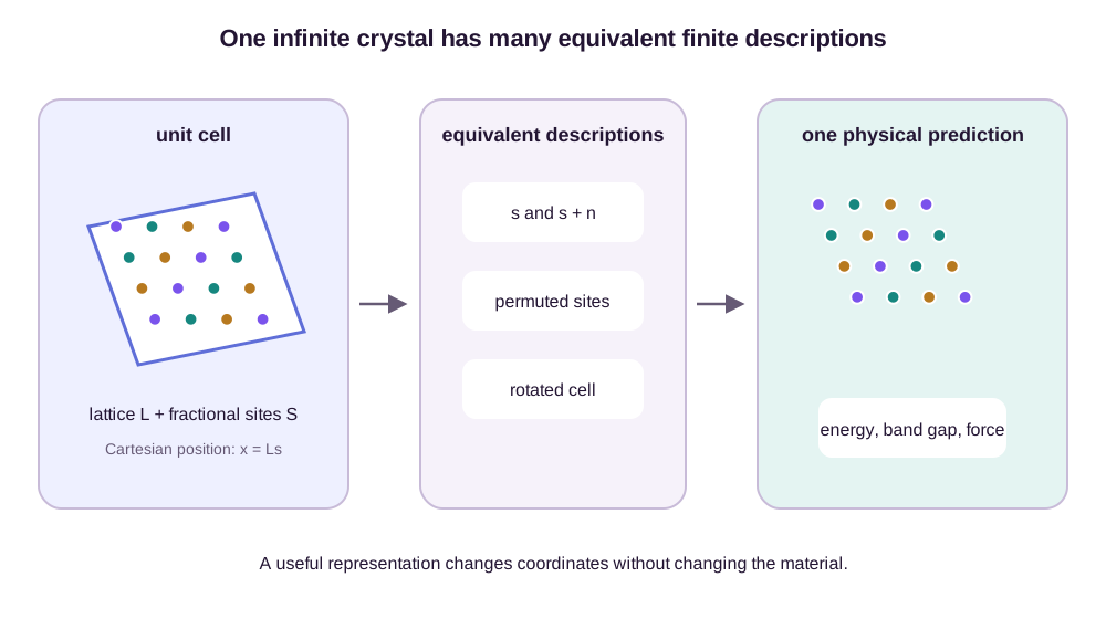
These are not optional augmentations. They define the quotient space on which learning occurs. Let \(\pi\) relabel sites, let \(Q\) be a rigid rotation, let \(M\in GL(3,\mathbb Z)\) be unimodular, let \(t\in\mathbb R^3\) be a common fractional origin shift, and let \(n_i\in\mathbb Z^3\). The complete fixed-site-count action is
\[z_i'=z_{\pi(i)}, \qquad L'=QLM, \qquad s_i'=M^{-1}(s_{\pi(i)}+t)+n_i.\]Indeed,
\[L's_i' =QL(s_{\pi(i)}+t)+QLMn_i,\]so the physical site is rotated by \(Q\), translated by the common Cartesian vector \(QLt\), and shifted only by a lattice image. For an intensive scalar property \(f\) such as formation energy per atom or band gap, the requirement is \(f(A',L',S')=f(A,L,S)\). Forces differ: after undoing site relabeling, their Cartesian vectors rotate by \(Q\). Non-unimodular supercells change site count and are handled separately below rather than included in this fixed-size action.
The companion post Materials Discovery Connects Structure, Properties, and Synthesis develops the broader scientific loop. Here the narrower concern is what periodic geometry permits a learned model to claim.
One crystal, two lattice bases
I will use one small layered crystal throughout. It is two-dimensional but embedded in three dimensions with vacuum along \(z\). Adopt a column-vector convention: lattice vectors are columns of
\[L= \begin{pmatrix} 2&0&0\\ 0&1&0\\ 0&0&6 \end{pmatrix},\]and fractional coordinates are column vectors. The cell contains A at \(s_A=(0,0,1/2)^{\mathsf T}\) and B at \(s_B=(3/4,1/4,1/2)^{\mathsf T}\). Their Cartesian positions are \((0,0,3)^{\mathsf T}\) and \((3/2,1/4,3)^{\mathsf T}\).
Change the stored lattice basis with the integer unimodular matrix
\[M= \begin{pmatrix} 1&1&0\\ 0&1&0\\ 0&0&1 \end{pmatrix}, \qquad M^{-1}= \begin{pmatrix} 1&-1&0\\ 0&1&0\\ 0&0&1 \end{pmatrix}, \qquad \det M=1.\]The same crystal is represented by
\[L'=LM, \qquad s_i'=M^{-1}s_i.\]The new second lattice vector is \(\ell_1+\ell_2=(2,1,0)^{\mathsf T}\), and B becomes \(s_B'=(1/2,1/4,1/2)^{\mathsf T}\). Cartesian positions are unchanged because
\[L's_i'=LMM^{-1}s_i=Ls_i.\]For B, the finite check is
\[L's_B' =\frac12(2,0,0)^{\mathsf T} +\frac14(2,1,0)^{\mathsf T} +\frac12(0,0,6)^{\mathsf T} =(3/2,1/4,3)^{\mathsf T}.\]This is a basis change, not a rigid rotation. Cartesian forces and stresses should therefore remain numerically unchanged. Fractional components transform: if a Cartesian vector is written \(v=Lu\), then its new fractional components are \(u'=M^{-1}u\). Under a separate rigid rotation \(Q\), Cartesian vectors transform as \(v\mapsto Qv\) and second-order tensors as \(T\mapsto QTQ^{\mathsf T}\).
| Intensive scalar outputs such as band gap or energy per atom are unchanged. An extensive energy for this unimodular cell is also unchanged because $$ | \det M | =1\(preserves volume and site count. A non-unimodular supercell transformation with determinant magnitude\)m\(would scale extensive cell energy and atom count by\)m$$ while leaving intensive quantities fixed. “Cell invariance” must say which output is being compared. |
Crystal Graphs Turn Periodicity into Local Neighborhoods
A crystal graph takes sites in a reference cell as nodes and connects atoms through nearby periodic images. For sites \(i\) and \(j\), an edge can carry the displacement
\[r_{ij,n}=L(s_j-s_i+n),\qquad n\in\mathbb Z^3,\]when \(\lVert r_{ij,n}\rVert\) lies below a cutoff. The integer image index \(n\) matters: two atoms on opposite faces of the displayed unit cell may be nearest neighbors in the infinite crystal. The graph is finite because only images within the cutoff are included.
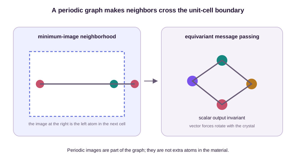
A message-passing predictor updates site features as
\[h_i^{(k+1)}=\phi\!\left(h_i^{(k)}, \sum_{j,n:\lVert r_{ij,n}\rVert<r_c} \psi\!\left(h_i^{(k)},h_j^{(k)},e(r_{ij,n})\right)\right),\]then pools sites to obtain a crystal representation. If \(e\) uses only distance expansions, the model is invariant to rigid rotations and reflections. This is sufficient for many scalar properties. CGCNN established this graph-based template for learning formation energies, band gaps, elastic quantities, and related properties directly from crystal structures (Xie and Grossman, 2018).
Distance-only messages nevertheless discard angular information unless several layers reconstruct it indirectly. Periodic equivariant networks instead maintain vector or higher-order geometric features. Under a rigid rotation \(Q\), a scalar feature remains unchanged while a vector feature transforms as \(v_i\mapsto Qv_i\). Equivariant coordinate or force updates can then use directional information without choosing a preferred laboratory frame.
The distinction matters most when the output is geometric. An energy model should be invariant, \(E(QX)=E(X)\). If forces are obtained consistently as \(F_i=-\nabla_{x_i}E\), then
\[F_i(QX)=QF_i(X).\]This gives the right behavior for relaxation and molecular dynamics. Space-group symmetry is more specific than global Euclidean symmetry: symmetry-equivalent sites should receive compatible features and forces. Encoding known space groups or Wyckoff positions can reduce redundancy, but an incorrectly imposed space group can also exclude a lower-symmetry phase.
The periodic edge survives the basis change
For the running cell, the nearest image of B seen from A uses \(n=(-1,0,0)^{\mathsf T}\). Its displacement is
\[r_{AB,n} =L(s_B-s_A+n) =L(-1/4,1/4,0)^{\mathsf T} =(-1/2,1/4,0)^{\mathsf T},\]with distance \(\sqrt{5}/4\approx0.559\). The unshifted B is about \(1.521\) away, and the image with \(n=(-1,-1,0)\) is about \(0.901\) away. Thus a cutoff \(r_c=0.8\) includes exactly the nearest A–B image among these candidates.
Image indices transform with the fractional coordinates. Set \(n'=M^{-1}n=(-1,0,0)^{\mathsf T}\). Then
\[\begin{aligned} r'_{AB,n'} &=L'(s_B'-s_A'+n')\\ &=LM\left[M^{-1}(s_B-s_A)+M^{-1}n\right]\\ &=L(s_B-s_A+n)=r_{AB,n}. \end{aligned}\]The stored fractional displacement changes from \((-1/4,1/4,0)\) to \((-1/2,1/4,0)\), yet multiplication by the changed lattice returns the same Cartesian edge. Keeping \(n\) fixed while changing basis happens to work for this particular vector, but it fails in general; the correct law is \(n'=M^{-1}n\). Neighbor enumeration must transform the whole integer image lattice, not only wrap sites into a displayed cell.
One periodic message update
Give A and B scalar features \(h_A=1\) and \(h_B=2\). Use the toy message \(m_{ij}=h_j\exp(-\lVert r_{ij}\rVert^2)\) and update \(h_i'=h_i+\sum_jm_{ij}\). The edge has squared length \(5/16\), so \(\exp(-5/16)\approx0.732\). The two updates are
\[h_A'=1+2(0.732)=2.464, \qquad h_B'=2+1(0.732)=2.732.\]Both lattice bases give these values because the Cartesian displacement is identical. A directional message such as \(h_jr_{ij}\) is also basis-independent in Cartesian coordinates and rotates covariantly under a physical rotation.
The cutoff still imposes a scientific boundary. At \(r_c=0.8\), no in-plane lattice image at distance 1 or more enters, and the \(6\)-unit vacuum removes interlayer images. More message-passing layers expand graph-hop reach only through edges that exist. They cannot reconstruct long-range electrostatics or an omitted interlayer interaction across a disconnected cutoff graph. Periodicity makes local neighborhoods correct; it does not make a local model globally complete.
Property Prediction Is Conditional on Structure and Data Provenance
For a known relaxed structure, a predictor approximates
\[\widehat y=f_\theta(A,L,S).\]This looks straightforward, but the target encodes a calculation protocol. Formation energies depend on reference states and density-functional settings. Band gaps inherit the systematic bias of the electronic-structure approximation. Magnetic configurations, disorder, temperature, pressure, and defects may be absent from the input even when they control the measurement.
Formation energy alone also does not determine stability against decomposition. For composition \(c\), stability is judged relative to competing phases through the energy above the convex hull,
\[E_{\mathrm{hull}}(c)=E(c)-\min_{\{\lambda_k\}} \sum_k\lambda_kE(c_k),\]subject to \(\lambda_k\ge 0\), \(\sum_k\lambda_k=1\), and \(\sum_k\lambda_kc_k=c\). A negative formation energy relative to elements can coexist with a positive hull distance because a mixture of compounds is lower in energy. The result is meaningful only relative to the phase set and calculation consistency used to build the hull.
Generalization is therefore chemical and structural, not merely random-split accuracy. A random split can place nearly identical compositions or prototypes in train and test sets. Performance on a new chemical system, pressure regime, or coordination motif can be substantially worse. Uncertainty estimates help triage expensive calculations, but they must be calibrated on the same kind of distribution shift that deployment will encounter.
Output laws on the running cell
A representation audit should include outputs, not only reconstructed coordinates. Suppose the predictor returns band gap \(2.4\), cell energy \(-5.0\), Cartesian forces
\[F_A=(1,-2,0)^{\mathsf T}, \qquad F_B=(-1,2,0)^{\mathsf T},\]and in-plane stress
\[T= \begin{pmatrix}3&1\\1&2\end{pmatrix}.\]The unimodular basis change must leave all four Cartesian quantities numerically unchanged because no physical object moved. Force A has old fractional components \(u_A=L^{-1}F_A=(1/2,-2,0)^{\mathsf T}\). Its new components are
\[u_A'=M^{-1}u_A=(5/2,-2,0)^{\mathsf T},\]and reconstruction gives \(L'u_A'=(1,-2,0)^{\mathsf T}\). Comparing fractional force arrays entrywise across bases would falsely report a violation; they are coordinate components and must transform.
Now apply a physical \(90^\circ\) rotation in the layer. With \(Q(x,y,z)=(-y,x,z)\), force A becomes \((2,1,0)^{\mathsf T}\). The in-plane stress becomes
\[QTQ^{\mathsf T} =\begin{pmatrix}2&-1\\-1&3\end{pmatrix},\]while band gap and energy remain \(2.4\) and \(-5.0\). These two tests diagnose different contracts: basis covariance changes stored components without moving the crystal, while Euclidean covariance moves the crystal in space.
Data provenance can hide the first failure. If every training file uses one standardized conventional cell, a network may exploit lattice-entry regularities and still score well. Evaluation should generate equivalent unimodular bases on held-out structures and compare the transformed outputs. Prototype- or composition-aware splits address chemical transfer; they do not test unit-cell gauge consistency.
Generation Moves Composition, Cell, and Sites Together
Crystal structure prediction with fixed composition seeks plausible \((L,S)\) given \(A\). Ab initio generation may move all three variables. They inhabit different spaces:
- element types and stoichiometric counts are discrete;
- a valid lattice is a continuous, nonsingular matrix modulo rotations and equivalent cell choices;
- fractional sites live on a three-dimensional torus because \(s_i\) and \(s_i+n\) are identical.
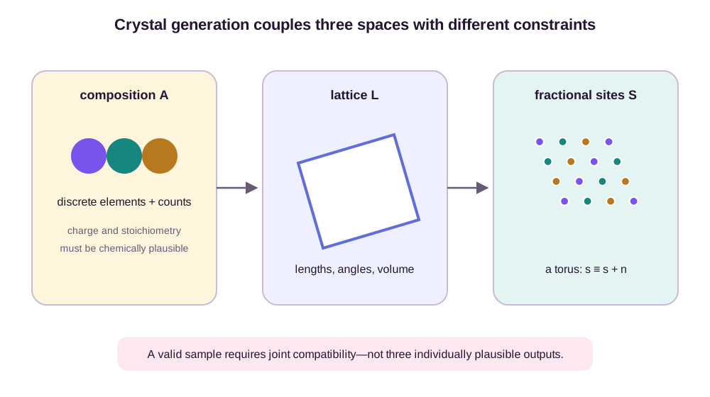
This coupling rules out a naive Cartesian generator. If coordinates are noised independently while the cell is generated separately, density and coordination can drift apart. If fractional coordinates are treated as ordinary Euclidean variables, sites near 0 and 1 appear far apart despite being adjacent on the torus. If atom counts change, the state dimension changes. If the cell matrix is parameterized without constraints, it can become singular or flip handedness.
CDVAE addressed periodic material generation with a latent variable for composition and lattice and a score-based decoder for atomic coordinates (Xie et al., 2022). Its conceptual factorization is useful: global variables propose the broad crystal, while a periodic decoder realizes atom positions. But reconstruction quality and latent smoothness do not by themselves establish thermodynamic stability.
DiffCSP instead formulates crystal structure prediction as joint equivariant diffusion of lattice and fractional coordinates conditioned on composition (Jiao et al., 2023). A schematic forward process is
\[L_t=\alpha_tL_0+\sigma_t\epsilon_L, \qquad s_{i,t}=(s_{i,0}+\sigma_t\epsilon_i)\bmod 1.\]The wrapped coordinate process respects periodicity; the denoiser must also preserve permutation and E(3) behavior. Flow matching offers a related construction: learn a time-dependent vector field carrying a simple base distribution to the data distribution. In either case, the interpolation path is part of the inductive bias. It determines what intermediate cells and sites the network must learn to repair.
For fixed composition AB, the discrete variable disappears but the state is still constrained. Fractional coordinates lie on \((\mathbb T^3)^2\), so adding noise must wrap each component. If B moves from \(s_x=0.98\) by \(+0.05\), the result is \(0.03\), not an out-of-range coordinate at \(1.03\) and not a long move across the cell. A score or velocity should be periodic in this coordinate; an ordinary Euclidean regression at the branch cut creates a false discontinuity.
The lattice needs a different constraint. Nonsingularity alone permits cells with vanishing thickness and extreme condition number. One safe parameterization generates a positive-definite Gram matrix \(G=L^{\mathsf T}L\) through a Cholesky factor with positive diagonal entries, then chooses a frame for \(L\). For the layered example, validity might require \(\det L>0\), in-plane singular values above \(0.5\), vacuum height above \(4\), density within a declared range, and minimum periodic A–B distance above \(0.3\). These thresholds define an accepted distribution; they are not consequences of diffusion.
The generator must also transform consistently under basis choice. A density on raw matrix entries \(p(L,S)\) can assign different likelihood to \((L,S)\) and \((LM,M^{-1}S)\) even though they represent the same crystal. Canonical reduction chooses one representative but introduces discontinuities where the chosen reduced basis changes. Basis augmentation averages over representatives but supplies only the invariance achieved by that averaging procedure. A quotient-aware objective or explicit consistency test should state which basis transformations it covers.
| For the declared unimodular transformation, the fractional-site map has Jacobian magnitude $$ | \det M^{-1} | =1\(per site. Right multiplication\)L\mapsto LM\(on a three-row lattice matrix has Jacobian\) | \det M | ^3=1$$. Thus no density correction is needed for this finite change of variables: a basis-consistent model should assign equal density to the two representatives. This statement does not extend unchanged to conventional-cell expansions, which alter atom count and state dimension rather than reparameterize the same fixed-size tuple. |
Symmetry Can Be Predicted, Conditioned, or Enforced
Space-group information offers a compact description of repeated structure. One strategy generates all sites and later identifies symmetry. Another conditions generation on a target space group. A stronger strategy generates only an asymmetric unit and expands it through space-group operations. If a site \(s\) occupies a Wyckoff position, the orbit
\[\mathcal O(s)=\{R_gs+t_g\bmod 1:g\in G\}\]produces all symmetry-equivalent sites under space group \(G\).
Enforcement guarantees exact symmetry and reduces the number of free coordinates. It can also make composition constraints delicate because Wyckoff multiplicities determine how many atoms appear. Conditioning is more flexible but can produce approximate symmetry that disappears after relaxation. Predicting symmetry from data risks treating inconsistent conventional-cell labels as physical differences.
The correct choice depends on the scientific question. Searching within a known high-symmetry family benefits from enforcement. Discovering symmetry-breaking distortions or low-temperature phases requires freedom to leave that family. Symmetry is a prior over the search space, not an unconditional guarantee of stability.
Multiplicity makes the composition constraint arithmetic. Consider the two-operation group on the layer generated by inversion, \(s\mapsto-s\bmod1\). A general site such as \((1/4,1/4,1/2)\) has orbit
\[\{(1/4,1/4,1/2),(3/4,3/4,1/2)\},\]so its Wyckoff multiplicity is two. The origin is fixed modulo the lattice and has multiplicity one. Placing A at the origin and one independent B at the general site produces AB\(_2\) after symmetry expansion, not AB. An exactly inversion-symmetric AB cell must put B on another multiplicity-one special position, such as \((1/2,0,1/2)\), or change the cell and symmetry description.
This is why “condition on composition AB and space group \(G\)” can be infeasible before coordinates are generated. The requested element counts must be partitionable into allowed Wyckoff multiplicities, including occupancies if disorder is admitted. A decoder that samples an asymmetric unit and repairs the count afterward changes its distribution. A decoder that rejects incompatible assignments should report the rejection denominator. Symmetry enforcement guarantees membership in the declared orbit construction, not that the declared composition and symmetry admit a low-energy crystal.
Property Guidance Creates an Oracle-Optimization Problem
Inverse design asks for crystals satisfying a target property \(y^*\). A conditional generator approximates \(p_\theta(A,L,S\mid y^*)\); classifier or energy guidance modifies a base generator using gradients of a learned oracle. MatterGen jointly denoises atom types, coordinates, and the lattice, and supports conditioning on composition, symmetry, and scalar properties (Zeni et al., 2025). Its experimental synthesis of a generated candidate is important precisely because generative and predictive scores are not the final evidence.
Guidance produces a familiar tradeoff. Stronger pressure toward a target can increase predicted performance while decreasing diversity and moving candidates outside the oracle’s training distribution. A model optimized for low predicted formation energy may repeat a narrow prototype family. A band-gap target may be satisfied according to a surrogate whose errors correlate with composition. Multi-objective design introduces further tension: stability, abundance, toxicity, conductivity, mechanical response, and processability rarely improve together.
The appropriate output is therefore a Pareto set rather than a single “best” crystal. Candidate \(u\) dominates \(v\) only if it is no worse on every objective and better on at least one. This leaves tradeoffs visible for subsequent calculations and experiments. Collapsing them into one weighted score hides value judgments and creates a sharper target for oracle exploitation.
A finite guided distribution
Take three fixed-composition AB candidates. Their learned prior masses, predicted target rewards, and predicted stability scores are
| candidate | prior \(p_0\) | target reward \(r\) | stability score | uncertainty \(\sigma_r\) |
|---|---|---|---|---|
| C1 | 0.60 | 0.6 | 0.9 | 0.1 |
| C2 | 0.30 | 1.2 | 0.7 | 0.2 |
| C3 | 0.10 | 2.0 | 0.2 | 0.8 |
An exponential guidance tilt gives \(p_\lambda(C)\propto p_0(C)e^{\lambda r(C)}\). At \(\lambda=1\), the unnormalized masses are approximately \((1.093,0.996,0.739)\) and the probabilities are \((0.386,0.352,0.261)\). At \(\lambda=3\), the masses become \((3.630,10.979,40.343)\) and the probabilities \((0.066,0.200,0.734)\). Strong guidance makes the rare, high-oracle C3 dominate exactly where its uncertainty is largest.
The three candidates are Pareto-nondominated in target reward and stability. A weighted score \(w r+(1-w)s\) with \(w=0.3\) gives \((0.81,0.85,0.74)\) and selects C2. With \(w=0.7\) it gives \((0.69,1.05,1.46)\) and selects C3. The optimizer has answered two different policy questions, not resolved the tradeoff.
Uncertainty can change the choice again. The conservative target score \(r-2\sigma_r\) is \((0.4,0.8,0.4)\), so C3 loses its apparent advantage. This penalty is only as credible as calibration on guided candidates. If the oracle and uncertainty ensemble share training data and architecture, they can agree on the same extrapolation error. Independent higher-fidelity calculations must evaluate a frozen selection rather than silently guide another round under the same budget.
Valid, Unique, Novel, Stable, and Useful Are Different Claims
Generative evaluation often reports validity, uniqueness, and novelty. Each requires a precise equivalence rule.
Validity may mean only parseable elements, a nonsingular cell, and no severe overlaps. Chemical validity additionally involves oxidation states, charge balance, coordination, and density. Uniqueness requires symmetry-aware structure matching; byte-distinct CIF files can encode the same crystal. Novelty depends on the database, tolerance, and whether comparison uses composition, prototype, or relaxed structure. A small distortion of a known phase can appear novel before relaxation and identical afterward.
Stability is yet another claim. A property predictor can screen formation energy, but relaxation may move the structure far from the generated geometry. DFT can locate a local minimum and estimate hull distance, but zero-temperature thermodynamic stability does not guarantee dynamical stability. Imaginary phonon modes indicate distortions along which the structure can lower its energy. Finite-temperature free energies, pressure, disorder, and metastable kinetic trapping can change the picture.
Finally, a stable crystal need not be synthesizable, and a synthesizable material need not be useful. Precursors, reaction pathways, competing phases, defects, particle size, processing, and environmental stability affect what the laboratory obtains. Device performance can depend on interfaces and microstructure absent from an ideal periodic cell.
Relaxation Is Part of Evaluation, Not Cosmetic Cleanup
A generated structure \(X_g=(A,L,S)\) is usually not at a local energy minimum. Relaxation iterates positions and often the cell using predicted or first-principles forces,
\[X^{(k+1)}=X^{(k)}-\eta_k\nabla_XE(X^{(k)}),\]until forces and stresses are small. Machine-learned interatomic potentials can screen many candidates cheaply; selected structures then receive density-functional theory (DFT) relaxation and property calculations.
The displacement between generated and relaxed structures is diagnostic. Small drift suggests that the generator proposed a basin near a local minimum. Large drift means the original coordination or cell was not self-consistent, even if the relaxed endpoint is valid. Reporting only the endpoint gives the generator credit for the optimizer’s repair. Conversely, rejecting every large-drift candidate can discard unusual but physically meaningful starting points. The threshold must match the intended claim.
Relaxation is many-to-one. Suppose raw proposals R1 and R2 are distinct distortions of the running AB structure, while R3 lies near another basin. A frozen surrogate gives
| raw proposal | raw target property | raw energy proxy | relaxed basin | relaxed target property | relaxed energy |
|---|---|---|---|---|---|
| R1 | 2.1 | -0.4 | X | 1.2 | -0.90 |
| R2 | 1.8 | -0.5 | X | 1.2 | -0.90 |
| R3 | 1.5 | -0.8 | Y | 1.4 | -0.85 |
Before relaxation, R1 ranks first on the target property and R3 ranks last. After relaxation, R1 and R2 collide into the same structure X, while Y from R3 has the largest target value. The raw set has three symmetry-distinct proposals but only two unique relaxed outcomes. A novelty calculation before relaxation can count R1 and R2 separately even though the energy landscape erases their distinction.
The collision changes denominators and attribution. If a screening policy sends only raw-property winner R1 to expensive relaxation, it returns property 1.2 and misses Y at 1.4. If both R1 and R2 are selected, two computational slots purchase one basin. A generator can still deserve credit for placing mass in X’s basin, but not for producing two distinct materials. Reports should retain raw coverage, relaxation convergence, post-relaxation uniqueness, basin multiplicity, displacement, and both pre- and post-relaxation property ranks.
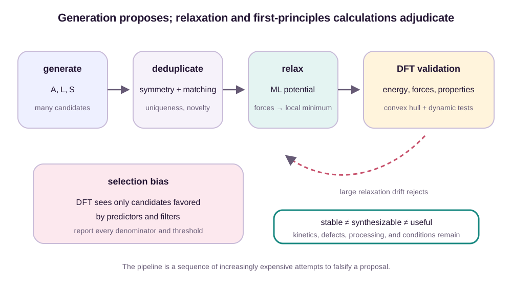
This funnel creates selection bias. Suppose one million samples are reduced to ten thousand by a learned stability model, one thousand by novelty and property filters, and one hundred by relaxation before DFT. The DFT success rate describes those hundred candidates, not the generator’s unconditional yield. It also cannot show whether a property oracle added value unless random or stratified candidates are calculated as controls.
A rigorous report preserves every denominator: raw samples, valid structures, symmetry-aware unique structures, database-novel structures, successfully relaxed structures, DFT-stable structures, target-property candidates, synthesis attempts, and characterized products. It records thresholds and failures, not only the final shortlist. Comparisons should use the same computational settings and reference phase diagram. Prospective experiments should fix the selection policy before outcomes are known.
A denominator-preserving campaign
Consider a declared campaign with the following frozen funnel:
| stage | survivors | conditional rate | rate from raw |
|---|---|---|---|
| generated AB proposals | 10,000 | — | 100% |
| valid lattice and density | 8,000 | 80.0% | 80.0% |
| minimum-distance and charge checks | 6,000 | 75.0% | 60.0% |
| symmetry-aware unique raw structures | 4,500 | 75.0% | 45.0% |
| learned-potential relaxation converged | 3,600 | 80.0% | 36.0% |
| unique relaxed basins | 2,400 | 66.7% | 24.0% |
| selected under frozen uncertainty/Pareto rule | 400 | 16.7% | 4.0% |
| DFT relaxation converged | 320 | 80.0% | 3.2% |
| stable under declared calculation and phase set | 80 | 25.0% | 0.8% |
| target property after DFT | 30 | 37.5% | 0.3% |
| synthesis attempts | 12 | 40.0% | 0.12% |
| phase-confirmed products | 5 | 41.7% | 0.05% |
| characterized target hits | 2 | 40.0% | 0.02% |
The table reports 25% stability among DFT-relaxed candidates and 0.8% stability among raw proposals. Both are correct, but they support different claims. The first evaluates a selected computational shortlist. The second evaluates unconditional yield through the declared funnel. Two final hits correspond to 40% of phase-confirmed products, 16.7% of attempted syntheses, and 0.02% of generated proposals.
Every transformation must retain its own failure category. The reduction from 3,600 converged relaxations to 2,400 basins is not “failed relaxation”; it is a 1,200-count collision under the post-relaxation equivalence rule. The reduction from 2,400 to 400 is a policy decision, not physical invalidity. Candidates outside the 400 remain unevaluated at DFT fidelity. Calling them unstable would turn missing evidence into a negative label.
The broader materials-discovery chapter develops convex-hull construction, defects, finite-temperature rankings, process windows, and experimental characterization. This chapter’s interface contract is narrower:
| reported claim | required denominator and evidence |
|---|---|
| representation consistency | equivalent cells, including unimodular basis changes, give matching invariant outputs and transformed vector/tensor outputs |
| proposal coverage | raw samples measured against a declared reference distribution or held-out structures before repair |
| valid-generation rate | all raw proposals, with every lattice, distance, composition, and symmetry rejection counted |
| relaxed structural yield | all raw proposals plus convergence and post-relaxation collision counts |
| predicted-property enrichment | frozen selected and control strata evaluated by an independent property calculation |
| thermodynamic stability | named phase set, electronic-structure protocol, and conditions, reported for every DFT-evaluated candidate |
| synthesis success | all attempted candidates and routes, including failures and phase identity |
| application hit | all characterized products under a declared measurement protocol |
A prospective comparison should also reserve random or stratified controls from the 2,400 relaxed basins. Without them, 30 target-property candidates among 400 selected structures cannot show how much enrichment the guidance oracle supplied. Selection quality is the difference between frozen policies at a common evaluation budget, not the absolute quality of the chosen tail.
Generative Design Expands the Search, Not the Evidence
Periodic graphs and equivariant networks solve a foundational representation problem: physically equivalent cells should lead to equivalent predictions, and vector outputs should transform correctly. Diffusion and flow models then turn composition, lattice, and sites into movable design variables. Space groups can restrict the search; property models can guide it; relaxation can test whether a proposal sits near an energy minimum.
None of these steps collapses the materials pipeline into a single score. Property predictions inherit the coverage and approximation of their labels. Generated novelty depends on equivalence definitions. Stability is conditional on competing phases and thermodynamic conditions. DFT is evidence about an idealized model, not direct evidence of a synthesis route. Experimental success is conditional on every filter that selected the candidate.
The right role for crystal generation is therefore expansive but precise: propose coherent regions of chemical and structural space that conventional enumeration might miss, then submit those proposals to progressively more independent tests. The generator contributes imagination. Periodic geometry makes that imagination physically legible. Relaxation, first-principles calculations, and synthesis decide how much of it survives.
References
Xie, T. and Grossman, J. C. “Crystal Graph Convolutional Neural Networks for an Accurate and Interpretable Prediction of Material Properties.” Physical Review Letters 120, 145301 (2018). doi:10.1103/PhysRevLett.120.145301 ↩
Xie, T. et al. “Crystal Diffusion Variational Autoencoder for Periodic Material Generation.” International Conference on Learning Representations (2022). OpenReview ↩
Jiao, R. et al. “Crystal Structure Prediction by Joint Equivariant Diffusion.” Advances in Neural Information Processing Systems 36 (2023). Proceedings ↩
Zeni, C. et al. “A generative model for inorganic materials design.” Nature 639, 624–632 (2025). doi:10.1038/s41586-025-08628-5 ↩
Figure provenance: all four diagrams are original explanatory syntheses created for this post with scripts/generate_crystgen_figures.py. They reproduce no lecture, paper, or Flaticon assets and are released under CC BY 4.0 with the post.