Note: This post continues the statistical mechanics thread from Ensembles, Thermostats, and Barostats and From Jarzynski's Equality to Diffusion Models. The motivation comes partly from two recent projects from our group: TPS-DPS, which learns path-sampling bias forces without collective variables, and BioEmu-CV, which learns collective variables for enhanced sampling from a biomolecular foundation model.
Introduction
Molecular dynamics is easy to describe and hard to use. You have atoms, a potential energy function, and Newton’s equations. Integrate the equations for long enough, and the trajectory should tell you how the molecule moves. For background on molecular simulation, see Frenkel & Smit, 2001 and Tuckerman, 2010.
The phrase “long enough” hides the entire problem.
A femtosecond MD timestep resolves bond vibrations. Protein folding, ligand unbinding, conformational switching, and nucleation can take microseconds, milliseconds, or longer. The simulation spends nearly all its time vibrating inside one metastable basin and almost none of its time crossing the barrier that matters.
The key point for ML is that molecular simulation is not limited only by force-field accuracy or neural network speed. It is limited by sampling. A better potential energy model helps only if the dynamics visits the states whose probabilities, pathways, or free energies we need.
The sampling problem connects four ideas:
- Molecular dynamics samples trajectories from a path distribution.
- Enhanced sampling deliberately changes that path distribution to make rare events common.
- Collective variables define the low-dimensional coordinates where we apply the change.
- ML methods either learn better collective variables or bypass them by learning path-level bias forces directly.
The Jarzynski post developed the path-measure view: if we change the dynamics, we must account for the change in probability. Molecular simulation makes that accounting practical.
Molecular Dynamics Samples Paths
Consider atomic coordinates \(\mathbf{x} \in \mathbb{R}^{3N}\) and velocities \(\mathbf{v} \in \mathbb{R}^{3N}\). A potential energy function \(U(\mathbf{x})\) defines forces:
\[\mathbf{F}(\mathbf{x}) = -\nabla_{\mathbf{x}} U(\mathbf{x})\]Plain molecular dynamics integrates Newton’s equations:
\[\frac{d\mathbf{x}}{dt} = \mathbf{v}, \qquad m\frac{d\mathbf{v}}{dt} = \mathbf{F}(\mathbf{x})\]In practice, most equilibrium biomolecular simulations use a thermostat. A common choice is Langevin dynamics:
\[d\mathbf{x}_t = \mathbf{v}_t dt\] \[m\,d\mathbf{v}_t = \mathbf{F}(\mathbf{x}_t)dt - \gamma m\mathbf{v}_t dt + \sqrt{2\gamma m k_{B}T}\,d\mathbf{W}_t\]The force term pulls the system downhill in potential energy. The friction term removes kinetic energy. The noise term injects thermal fluctuations. Together they preserve the Boltzmann distribution:
\[p(\mathbf{x}) \propto e^{-\beta U(\mathbf{x})}, \qquad \beta = \frac{1}{k_{B}T}\]This is already familiar to ML people: \(U(\mathbf{x})\) is an energy function, \(p(\mathbf{x})\) is an energy-based model, and Langevin dynamics is a sampler.
MD samples paths, not only configurations:
\[\tau = (\mathbf{x}_0, \mathbf{x}_1, \ldots, \mathbf{x}_T)\]The distribution over paths depends on the potential, thermostat, timestep, and boundary conditions. If you change any of those, you change the path measure. That is why non-equilibrium identities like Jarzynski’s equality matter: they tell us how to recover equilibrium quantities after intentionally changing the dynamics.
The Timescale Problem
The Boltzmann distribution gives high probability to low free-energy basins, but it does not guarantee fast movement between them. Two conformations can both have large equilibrium probability while being separated by a high barrier.
The transition rate often scales roughly like:
\[k \propto e^{-\beta \Delta F^\ddagger}\]where \(\Delta F^\ddagger\) is the free-energy barrier between basins. Increasing the barrier by only a few \(k_{B}T\) can slow transitions by orders of magnitude.

This creates two different goals that are easy to confuse.
Equilibrium sampling asks: what configurations have high Boltzmann probability? For this, we care about correct averages under \(p(\mathbf{x})\). We may not care whether the trajectory crosses barriers with the real physical rate.
Kinetic sampling asks: how does the system move between states? For this, we care about transition paths, rates, committors, and mechanisms. We cannot freely change the dynamics unless we know how to correct for it.
Enhanced sampling methods live between these goals. They change the simulation so rare events happen in finite compute time. The price is that the simulated trajectory no longer follows the original physical dynamics. The method is useful only if we can recover the quantity we actually want.
Enhanced Sampling Is Controlled Distribution Shift
Enhanced sampling adds a bias to make hard regions easier to visit. The simplest version modifies the potential:
\[U_{\text{bias}}(\mathbf{x}) = U(\mathbf{x}) + V(\mathbf{x})\]The biased simulation samples:
\[p_{\text{bias}}(\mathbf{x}) \propto e^{-\beta (U(\mathbf{x}) + V(\mathbf{x}))}\]If \(V\) penalizes already-visited basins or lowers barriers, the trajectory explores more broadly. But now the samples come from the wrong distribution.
For equilibrium averages, the correction is importance weighting:
\[\langle A \rangle = \frac{\left\langle A(\mathbf{x}) e^{\beta V(\mathbf{x})} \right\rangle_{\text{bias}}}{\left\langle e^{\beta V(\mathbf{x})} \right\rangle_{\text{bias}}}\]This is the same logic as off-policy evaluation. You sample from one distribution because it is convenient, then correct back to the target distribution using a density ratio.
For path quantities, the correction involves ratios between path measures rather than configuration densities. That was the main point of the Jarzynski post. AIS, Jarzynski, Crooks, diffusion-model likelihoods, and transition-path objectives all ask the same question: how did changing the process change the probability of the whole trajectory?
Collective Variables
We cannot bias directly in \(3N\) coordinates. A protein with 1,000 atoms already has 3,000 coordinate dimensions. Depositing a useful bias in that space is hopeless.
Enhanced sampling therefore uses a collective variable:
\[s = \xi(\mathbf{x}) \in \mathbb{R}^{d}, \qquad d \ll 3N\]A CV is a low-dimensional summary of the molecular configuration. It might be a distance, angle, dihedral, contact count, radius of gyration, RMSD to a reference structure, or a learned neural representation.
For a molecular example, alanine dipeptide is the standard toy system. Its backbone conformation is often summarized by two dihedral angles:
\[s(\mathbf{x}) = (\phi(\mathbf{x}), \psi(\mathbf{x}))\]The contrast matters: a CV is not just any low-dimensional projection. Random atom coordinates can be low-dimensional but still fail to organize the slow states you care about.
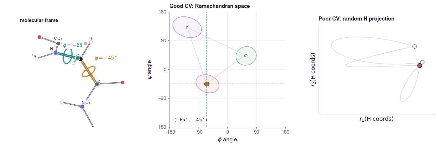
The free energy along the CV is:
\[F(s) = -\beta^{-1}\log p(s) + C\]where:
\[p(s) = \int \delta(s - \xi(\mathbf{x}))\,p(\mathbf{x})\,d\mathbf{x}\]The additive constant \(C\) is arbitrary. Only differences in \(F(s)\) matter.

A good CV should satisfy two conditions.
First, it should distinguish the metastable states we care about. If folded and unfolded proteins map to the same \(s\), biasing \(s\) cannot help.
Second, it should capture the slow mode of the transition. A coordinate can distinguish endpoints while missing the bottleneck between them. In that case, the simulation moves quickly along the CV but remains trapped in hidden orthogonal degrees of freedom. This is the classic failure mode: the projected free-energy profile looks flat, but the actual molecular system is still stuck.
CV discovery is therefore not ordinary dimensionality reduction. PCA finds high-variance directions. Many useful CVs are low-variance but slow. The relevant question is not “which coordinate explains the most variance?” but “which coordinate preserves the long-timescale dynamics?”
Umbrella Sampling
Umbrella sampling is the cleanest CV-based method (Torrie & Valleau, 1977). Choose windows centered at different CV values \(s_1, \ldots, s_K\). In window \(k\), add a harmonic bias:
\[V_k(\mathbf{x}) = \frac{1}{2}\kappa(\xi(\mathbf{x}) - s_k)^2\]Each window forces the simulation to explore a local region of the CV. The windows overlap. After collecting samples from all windows, methods such as WHAM or MBAR stitch the biased histograms together to estimate the unbiased free-energy profile.
The ML analogy is stratified sampling. Instead of hoping the Markov chain visits rare CV regions on its own, we force coverage of each region and correct afterward.
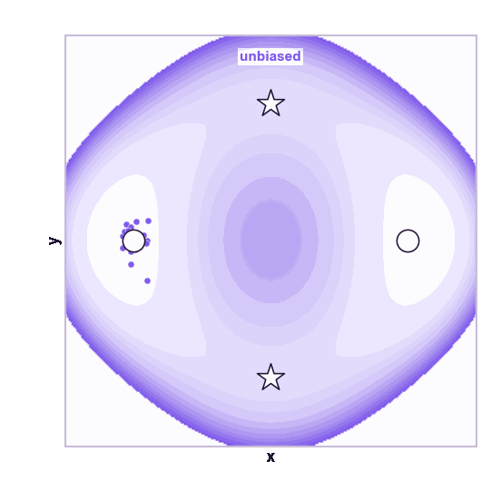
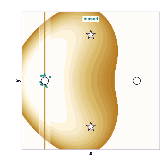
The same toy system makes the sampling effect visible. The next animations show illustrative overdamped dynamics, not a calibrated molecular timestep.
The weakness is that umbrella sampling requires planning. You need a CV, window centers, force constants, and enough overlap. If the transition coordinate is unknown or curved, the windows can miss the important path.
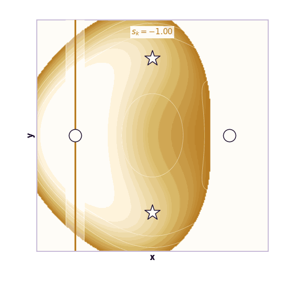
Metadynamics
Metadynamics automates part of this process (Laio & Parrinello, 2002). Instead of fixing windows ahead of time, it builds a history-dependent bias during the simulation.
At time \(t\), suppose the current CV value is \(s_t = \xi(\mathbf{x}_t)\). Metadynamics deposits a small Gaussian hill centered at \(s_t\):
\[V_t(s) = \sum_{t_i < t} w_i \exp\!\left(-\frac{\lVert s - s_{t_i}\rVert^2}{2\sigma^2}\right)\]The system is discouraged from returning to places it has already visited. Over time, the bias fills free-energy wells and pushes the simulation across barriers.

In ordinary metadynamics, the accumulated bias approaches:
\[V(s) \approx -F(s)\]up to an additive constant. In well-tempered metadynamics (Barducci et al., 2008), the hill heights decay so the bias approaches a scaled version of \(-F(s)\). This improves stability and makes reweighting better behaved.
Metadynamics is popular because it is intuitive: fill the holes until the landscape is flat. It also exposes the central dependency of enhanced sampling. If the CV is good, metadynamics can turn impossible transitions into routine ones. If the CV is bad, it confidently fills the wrong landscape.
Steered MD and Transition Paths
Umbrella sampling and metadynamics usually target equilibrium free-energy profiles. Sometimes we want the transition path itself: how a molecule goes from state A to state B.
Steered molecular dynamics (SMD) pulls the system along a CV according to a schedule:
\[V(\mathbf{x}, t) = \frac{1}{2}\kappa(\xi(\mathbf{x}) - s(t))^2\]This creates non-equilibrium trajectories. The work done by the moving restraint can be used with Jarzynski’s equality (Jarzynski, 1997):
\[\left\langle e^{-\beta W} \right\rangle = e^{-\beta \Delta F}\]This is the practical side of the Jarzynski post. We deliberately drive the system out of equilibrium because waiting for spontaneous transitions is too expensive. The driven trajectories are biased, but the path-measure ratio contains the correction.
The problem is variance. Jarzynski is exact, but the exponential average is dominated by rare low-work trajectories. Most fast pulls dissipate too much work. In ML terms, the estimator is unbiased but can be unusable.
Modern rare-event methods try to learn better proposals for this reason. We do not only want a force that reaches state B. We want a path distribution close to the true transition-path distribution, so the importance weights or path-measure corrections have manageable variance.
Where ML Enters
ML enters in two places. The first is to learn the CV: train a neural network coordinate \(s = \xi(\mathbf{x})\) that preserves slow dynamics, separates metastable states, or approximates committor-like information. Time-lagged objectives for slow molecular coordinates have a long history (Perez-Hernandez et al., 2013). In our group, BioEmu-CV (Park et al., 2025) learns such CVs from a biomolecular ensemble generator. The goal is not to replace enhanced sampling. It is to provide a better coordinate for methods such as OPES or steered MD.
The second entry point is to learn the path bias directly. Instead of choosing a low-dimensional CV first, train forces or proposals that make transition paths more likely while keeping track of the path distribution being sampled. TPS-DPS, also from our group, follows this route with a diffusion path sampler (Seong et al., 2025). These projects illustrate the two design choices above: learn where to bias, or learn the path-level bias itself.

These routes are complementary, not mutually exclusive. Learning CVs keeps the classical machinery interpretable and reusable, but a low-dimensional CV can miss hidden barriers. Learning path biases removes that bottleneck, but the model must learn a whole trajectory distribution rather than a coordinate.
The Bias Is Not the Answer
Enhanced sampling can produce beautiful movies that are physically misleading. A biased trajectory is not evidence that the unbiased system would move that way.
The object to trust is not the biased trajectory itself. It is one of:
- an unbiased equilibrium estimate recovered by reweighting,
- a free-energy profile along a CV,
- a transition-path ensemble with controlled path weights,
- or a proposal distribution that improves sampling efficiency while preserving a correction formula.
This distinction matters for ML papers. If a model generates plausible conformational transitions, ask what distribution those paths come from. Are they equilibrium samples? Transition paths conditioned on endpoints? Steered paths? Diffusion samples from a learned prior? The answer determines which physical claims are valid.
The same warning applies to CVs. A learned coordinate can separate states and still fail as an enhanced-sampling CV. The test is not visualization quality. The test is whether biasing that coordinate improves sampling and whether the resulting estimates agree after reweighting or independent validation.
A Practical Checklist
When reading or designing an MD-plus-ML method, I find the following questions more useful than method names.
What is the target distribution? Is the goal the Boltzmann distribution over configurations, a free-energy difference, a transition-path distribution, or a kinetic rate?
What distribution is actually sampled? Unbiased MD, metadynamics, umbrella windows, steered trajectories, diffusion paths, and neural proposals all sample different objects.
What is the correction? For biased equilibrium sampling, look for reweighting. For non-equilibrium switching, look for work identities or path-measure ratios. For learned samplers, look for likelihoods, importance weights, or validation against unbiased reference data.
Where is the low-dimensional assumption? CV-based methods make it explicit through \(s = \xi(\mathbf{x})\). Path-based neural methods may avoid explicit CVs, but they still impose architectural and training biases.
What fails when the CV is wrong? Good papers show diagnostics: hysteresis, inconsistent free energies across runs, poor overlap between windows, hidden barriers, or transition paths that collapse to one mechanism.
Closing
Molecular dynamics gives us a physically grounded path distribution. Rare events make that distribution hard to sample. Enhanced sampling changes the distribution so useful events happen more often. Collective variables decide where the change is applied. Reweighting and path-measure identities decide what we can recover afterward.
A diffusion model, an AIS chain, a metadynamics run, and a transition path sampler all change a sampling process. The question is the same in each case: what path distribution did we sample, and how does it relate to the one we wanted?
The ML opportunity is larger than faster MD: change the sampling distribution while keeping the correction honest.
References
- Frenkel, D. & Smit, B. (2001). Understanding Molecular Simulation: From Algorithms to Applications. Academic Press. ↩
- Tuckerman, M. E. (2010). Statistical Mechanics: Theory and Molecular Simulation. Oxford University Press. ↩
- Torrie, G. M. & Valleau, J. P. (1977). Nonphysical sampling distributions in Monte Carlo free-energy estimation: umbrella sampling. J. Comput. Phys. 23, 187. ↩
- Laio, A. & Parrinello, M. (2002). Escaping free-energy minima. PNAS 99, 12562. ↩
- Barducci, A., Bussi, G. & Parrinello, M. (2008). Well-tempered metadynamics: a smoothly converging and tunable free-energy method. Phys. Rev. Lett. 100, 020603. ↩
- Jarzynski, C. (1997). Nonequilibrium equality for free energy differences. Phys. Rev. Lett. 78, 2690. ↩
- Perez-Hernandez, G. et al. (2013). Identification of slow molecular order parameters for Markov model construction. J. Chem. Phys. 139, 015102. ↩
- Seong, K., Park, S., Kim, S., Kim, W. Y. & Ahn, S. (2025). Transition Path Sampling with Improved Off-Policy Training of Diffusion Path Samplers. ICLR 2025. ↩
- Park, S., Seong, K., Yang, S., Gomez-Bombarelli, R. & Ahn, S. (2025). Learning Collective Variables for Enhanced Sampling from BioEmu with Time-Lagged Generation. arXiv:2507.07390. ↩