On this page
Adapted from my 2025 Machine Learning for Molecules lectures. This article explains the physical choices that determine what a molecular model can represent, predict, and conserve.
Molecular machine learning has an unusual constraint: its inputs are human-made descriptions, but its targets belong to a physical system that does not care how we describe it. Water has the same energy if we rotate the laboratory, rename its atoms, or translate it across the room. A crystal remains the same infinite solid if we choose a different but equivalent unit cell. A drug can have the same bond graph as its mirror image and still interact differently with a protein.
The central problem is therefore not simply to map an input vector to an output. We must decide which physical information enters the input, which transformations should leave the output unchanged, and which approximation defines the target. Those decisions form a chain:
\[\text{representation} \longrightarrow \text{electronic energy} \longrightarrow \text{force} \longrightarrow \text{ensemble} \longrightarrow \text{dynamics}.\]Each arrow removes detail while preserving the quantities needed at the next scale. Quantum mechanics turns nuclear identities and coordinates into an energy. Differentiation turns the energy into forces. Statistical mechanics turns energies into probabilities. Dynamics turns forces and thermal noise into trajectories. Most molecular ML tasks replace one expensive arrow in this chain.
A molecule has several valid representations
A molecule is a set of nuclei and electrons, but most datasets do not store its quantum state. They store a representation chosen for a particular prediction problem. The useful question is not which representation is most realistic. It is which distinctions the target depends on.
A representation is a controlled loss of information
Let \(x\) denote a physical molecular state and let \(\phi(x)\) be the representation passed to a model. Any representation groups together all states that produce the same encoded value:
\[[x]_{\phi}=\{x' : \phi(x')=\phi(x)\}.\]The set \([x]_{\phi}\) is the representation’s ambiguity class. A target \(y(x)\) can be predicted exactly from \(\phi(x)\) only if it is constant on every such class. If two states satisfy \(\phi(x_1)=\phi(x_2)\) but \(y(x_1)\neq y(x_2)\), no larger network or longer training run can repair the missing distinction. The best deterministic predictor must compromise between incompatible labels.
This statement separates representation error from model error. Suppose a dataset contains two conformers with the same molecular graph but energies \(0\) and \(8\) kJ/mol. A graph-only model receives the same input for both. Under squared loss with the two conformers weighted equally, its optimal prediction is their conditional mean, \(4\) kJ/mol, and the irreducible mean squared error is
\[\frac{(0-4)^2+(8-4)^2}{2}=16\;\text{(kJ/mol)}^2.\]The calculation does not say graphs are poor representations. It says a graph is insufficient for a conformation-specific energy. The same graph may be entirely adequate for a label that depends only on connectivity.
Strings, graphs, and coordinates discard different distinctions
A string representation such as SMILES records a traversal of a molecular graph (Weininger, 1988). For example, ethanol can be written as CCO. The same graph admits many valid SMILES strings because graph traversal is not unique. Canonicalization chooses one string by an algorithmic convention; it does not create a physical ordering of the atoms. InChI takes a different route: it constructs standardized layers for connectivity, charge, stereochemistry, isotopes, and related information (Heller et al., 2015). Both formats are compact and searchable. Both expose a molecule to a sequence model through a serialization that nature never supplied.
A molecular graph removes most of that serialization. Let \(G=(V,E)\) denote a graph with atoms \(i\in V\) and bonds \((i,j)\in E\). Node features can store atomic number, formal charge, and aromaticity; edge features can store bond order. A message-passing network then has a natural permutation symmetry: relabeling the atoms should relabel the hidden states but should not change a molecular property. Graphs work well when connectivity carries most of the signal. They are weaker when geometry controls the target.
Three-dimensional coordinates add that geometry. A conformation with \(N\) atoms can be written as atomic numbers \(\mathbf{z}=(z_1,\ldots,z_N)\) and positions \(\mathbf{R}=(\mathbf{r}_1,\ldots,\mathbf{r}_N)\), where \(\mathbf{r}_i\in\mathbb{R}^3\). The same graph can have many conformations because single bonds rotate and rings flex. Those conformations can have different energies, reactivities, and binding affinities. A 2D graph may say that two atoms are connected through four bonds; their 3D coordinates reveal whether they are actually close in space.
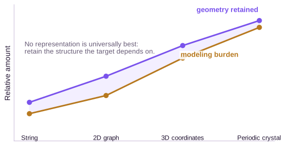
The hierarchy in the following figure is a modeling tradeoff, not a ranking. Richer geometric inputs can support richer targets, but they also require conformer generation, symmetry-aware architectures, and decisions about boundary conditions.
Chirality gives a sharp example of lost information. A chiral molecule and its mirror image are called enantiomers when no rotation and translation can superimpose them. They have the same ordinary bond graph and nearly all the same bulk scalar properties in an achiral environment. Yet a chiral receptor can distinguish them because reflection changes the handed arrangement of binding groups. Stereochemical annotations such as @ and @@ in isomeric SMILES recover this distinction at specified centers. A graph without those annotations does not.
Coordinates do not automatically preserve chirality if the model reduces them to pairwise distances. Consider three displacement vectors from a tetrahedral center, \(\mathbf{a}\), \(\mathbf{b}\), and \(\mathbf{c}\). Their handedness is measured by the signed volume
\[\chi=\det[\mathbf{a}\;\mathbf{b}\;\mathbf{c}] =\mathbf{a}\cdot(\mathbf{b}\times\mathbf{c}).\]For the simple coordinates \(\mathbf{a}=(1,0,0)\), \(\mathbf{b}=(0,1,0)\), and \(\mathbf{c}=(0,0,1)\), we obtain \(\chi=+1\). Reflecting through the \(yz\) plane sends \(\mathbf{a}\) to \((-1,0,0)\) and gives \(\chi=-1\). Every pairwise distance remains unchanged because an orthogonal reflection preserves norms. A distance-only representation therefore places the two configurations in the same ambiguity class even though a chiral environment can assign them different binding energies.
Periodic structure adds equivalences of its own
Crystals require one more piece of structure: periodicity. A periodic crystal can be represented by a lattice matrix \(\mathbf{L}\in\mathbb{R}^{3\times 3}\), fractional coordinates \(\mathbf{s}_i\in[0,1)^3\), and atomic numbers \(z_i\). The corresponding infinite set of nuclear positions is
\[\mathcal{C} = \left\{ (z_i,\,\mathbf{L}(\mathbf{s}_i+\mathbf{n})) \;:\; i=1,\ldots,N,\quad \mathbf{n}\in\mathbb{Z}^3 \right\}.\]The finite list inside one cell generates the infinite crystal through integer translations. The representation is not unique: shifting the origin, wrapping an atom into a neighboring cell, or choosing another primitive basis can describe the same crystal. Defects further complicate the picture. A vacancy, dopant, dislocation, or surface breaks the ideal periodic symmetry and may control the property of interest. A model trained only on perfect primitive cells cannot infer defect physics that never enters its input.
Symmetry tells a model what should change
Symmetry is a relation between transformations of the input and transformations of the output. Let \(g\) be a transformation such as a rotation or atom permutation, and let \(f\) be a predictor. A scalar predictor is invariant when
\[f(g\cdot x)=f(x).\]Energy is invariant to rigid translation, rigid rotation, and permutation of identical atoms. A vector predictor is equivariant when its output transforms with the input:
\[f(g\cdot x)=g\cdot f(x).\]Forces are equivariant to rotations: rotate every coordinate and every predicted force should rotate by the same matrix. This distinction is the organizing principle behind geometric deep learning (Bronstein et al., 2021).
An invariant energy forces an equivariant gradient
The energy-to-force relation turns a symmetry statement into a testable differential constraint. Let \(\mathbf{Q}\in SO(3)\) be a rotation and apply it to every atomic coordinate. Rotational invariance requires
\[E(\mathbf{Q}\mathbf{R})=E(\mathbf{R}),\]where \(\mathbf{Q}\mathbf{R}\) denotes the coordinate list \((\mathbf{Q}\mathbf{r}_1,\ldots,\mathbf{Q}\mathbf{r}_N)\). Differentiate both sides with respect to \(\mathbf{r}_i\). The chain rule introduces \(\mathbf{Q}^{\top}\):
\[\mathbf{Q}^{\top}\nabla_{\mathbf{Q}\mathbf{r}_i}E(\mathbf{Q}\mathbf{R}) =\nabla_{\mathbf{r}_i}E(\mathbf{R}).\]Multiplying by \(\mathbf{Q}\) and using \(\mathbf{F}_i=-\nabla_{\mathbf{r}_i}E\) gives
\[\mathbf{F}_i(\mathbf{Q}\mathbf{R}) =\mathbf{Q}\mathbf{F}_i(\mathbf{R}).\]Force equivariance is therefore not an additional preference when forces come from an invariant energy. It follows from the chain rule. A ninety-degree rotation around the \(z\) axis maps a force \((2,0,0)\) to \((0,2,0)\); an architecture that instead returns \((2,0,0)\) in both orientations violates the derivative of its own supposed energy law.
Translation invariance yields another exact check. Translate all atoms by the same vector \(\mathbf{t}\) and differentiate \(E(\mathbf{r}_1+\mathbf{t},\ldots,\mathbf{r}_N+\mathbf{t})=E(\mathbf{R})\) at \(\mathbf{t}=\mathbf{0}\):
\[\sum_{i=1}^{N}\nabla_{\mathbf{r}_i}E(\mathbf{R})=\mathbf{0}, \qquad \sum_{i=1}^{N}\mathbf{F}_i(\mathbf{R})=\mathbf{0}.\]An isolated molecule cannot acquire a net internal force. Rotation invariance similarly implies zero net internal torque, \(\sum_i \mathbf{r}_i\times\mathbf{F}_i=\mathbf{0}\), when coordinates are measured from a common origin. These identities are useful numerical diagnostics for learned potentials, not merely aesthetic properties.
Output type determines the constraint
The transformation law depends on the object being predicted. A molecular energy belongs to the trivial representation: every rotation acts as the number \(1\). A dipole moment belongs to the ordinary three-dimensional vector representation. A polarizability is a rank-two tensor and transforms as \(\boldsymbol{\alpha}\mapsto\mathbf{Q}\boldsymbol{\alpha}\mathbf{Q}^{\top}\) under a rotation matrix \(\mathbf{Q}\). Calling all three outputs “rotation-aware” hides the essential difference. The network must know not only that a symmetry exists, but also how each feature type transforms under it. The spherical equivariant layers article develops this representation-theoretic construction in detail.
Reflection requires care. Ordinary energies are unchanged by reflection when no external chiral field is present, but a pseudoscalar changes sign under reflection. Chirality-sensitive tasks may therefore need representations of parity, not just distances. Pairwise distances are invariant under every rotation and reflection, so they cannot distinguish enantiomers on their own. Angular and higher-order geometric features can carry more structure, provided the architecture treats parity consistently.
Molecular point groups collect rotations, reflections, and inversions that leave a finite geometry unchanged. Crystal space groups combine point operations with translations, including screw rotations and glide reflections. These symmetries constrain physical properties. For example, a structure with inversion symmetry cannot have a permanent electric dipole: inversion would reverse the dipole vector while leaving the structure unchanged, so the only consistent vector is zero. Symmetry is thus more than data augmentation. It can make some targets identically forbidden.
Electronic structure defines the energy landscape
Once the nuclei and their geometry are specified, quantum mechanics connects structure to energy. For a stationary state, the time-independent Schrödinger equation is
\[\hat{H}\Psi = E\Psi,\]where \(\hat{H}\) is the Hamiltonian operator, \(\Psi\) is the many-particle wavefunction, and \(E\) is an allowed energy. The equation is an eigenvalue problem over functions rather than finite vectors. For \(N_e\) electrons, the spatial part of \(\Psi\) depends on \(3N_e\) electron coordinates, before spin is included. Its squared magnitude gives a joint probability density over all electron configurations, not the probability of one unnamed electron at one point.
The hydrogen atom is the canonical exact solution because it contains one electron in a Coulomb potential. Separation in spherical coordinates produces orbitals labeled by quantum numbers. The familiar \(s\), \(p\), \(d\), and \(f\) labels correspond to orbital angular momentum values \(\ell=0,1,2,3\). These orbitals are not little paths followed by electrons. They are components of a quantum state whose amplitudes determine measurement probabilities.
Chemistry becomes difficult when electrons interact. In atomic units, and with the nuclei temporarily fixed, the electronic Hamiltonian is
\[\hat{H}_{e}(\mathbf{R}) = -\frac{1}{2}\sum_{i=1}^{N_e}\nabla_i^2 -\sum_{i=1}^{N_e}\sum_{A=1}^{N_n} \frac{Z_A}{\lvert\mathbf{r}_i-\mathbf{R}_A\rvert} +\sum_{i<j}\frac{1}{\lvert\mathbf{r}_i-\mathbf{r}_j\rvert} +\sum_{A<B}\frac{Z_AZ_B}{\lvert\mathbf{R}_A-\mathbf{R}_B\rvert}.\]Here \(\mathbf{r}_i\) and \(\mathbf{R}_A\) denote electron and nuclear positions, while \(Z_A\) is a nuclear charge. The four terms are electron kinetic energy, electron–nucleus attraction, electron–electron repulsion, and nucleus–nucleus repulsion. Electron–electron repulsion couples all electron coordinates, which prevents the equation from separating into independent one-electron problems.
The fixed nuclei in this Hamiltonian reflect the Born–Oppenheimer approximation (Born & Oppenheimer, 1927). Nuclei move much more slowly than electrons because nuclei are much heavier. The approximation turns that qualitative statement into a separation between electronic and nuclear motion.
Why mass produces a timescale separation
The mass argument can be made quantitative with the harmonic oscillator. For a coordinate with effective stiffness \(k\) and mass \(m\), the angular frequency is
\[\omega=\sqrt{\frac{k}{m}}.\]If an electronic and a nuclear coordinate experienced comparable curvature, their frequency ratio would scale as \(\omega_e/\omega_n\sim\sqrt{M/m_e}\). For a proton, \(M/m_e\approx1836\), so the ratio is about \(43\). The electronic coordinate responds through dozens of oscillations during one comparable nuclear period. Carbon nuclei increase the ratio by another factor of \(\sqrt{12}\). This is a scale estimate rather than a proof: electronic and nuclear curvatures are not generally equal, but the square-root mass dependence explains why an adiabatic separation is often plausible.
To see where the approximation enters, expand the full molecular wavefunction in electronic eigenstates that depend parametrically on nuclear geometry:
\[\Psi_{\mathrm{mol}}(\mathbf{r},\mathbf{R}) =\sum_n \chi_n(\mathbf{R})\,\psi_n(\mathbf{r};\mathbf{R}).\]Here \(\mathbf{r}\) collects electronic coordinates, \(\psi_n\) is the \(n\)th electronic state at fixed nuclei, and \(\chi_n\) is its nuclear amplitude. Applying the nuclear kinetic operator differentiates both factors. The product rule produces terms containing the derivative coupling
\[\mathbf{d}_{mn,A}(\mathbf{R}) =\left\langle\psi_m(\mathbf{R}) \middle| \nabla_{\mathbf{R}_A}\psi_n(\mathbf{R}) \right\rangle.\]The Born–Oppenheimer approximation neglects couplings between different electronic surfaces and keeps one term, usually the ground state. This is the non-obvious step: fixed nuclei are not an exact property of the Hamiltonian but the result of dropping nuclear-derivative couplings. Those couplings become large when electronic energy gaps shrink, which is why conical intersections, photochemistry, and charge-transfer events can require nonadiabatic dynamics.
With one electronic surface retained, the nuclear state evolves under the scalar energy below.
\[E_0(\mathbf{R}) = \min_{\Psi} \frac{\langle\Psi\mid\hat{H}_{e}(\mathbf{R})\mid\Psi\rangle} {\langle\Psi\mid\Psi\rangle}.\]The function \(E_0(\mathbf{R})\) is a potential energy surface (PES). It compresses electronic motion into an energy landscape for the nuclei. The approximation can fail near intersections between electronic states, during photoexcitation, and whenever electron and nuclear motion become strongly coupled. Within its usual regime, it is the bridge from electronic structure to molecular simulation.
The minimization expression also explains why an approximate electronic energy is usually an upper bound. For any normalized trial wavefunction \(\widetilde{\Psi}\),
\[\langle\widetilde{\Psi}\mid\hat{H}_{e}\mid\widetilde{\Psi}\rangle \ge E_0.\]This is the variational principle. Electronic-structure methods choose a tractable family of trial functions and optimize within it (Szabo & Ostlund, 1996). A richer family can lower the variational energy, but it also increases computation. The analogy to ML is close but incomplete: the ansatz is like an architecture, while the electronic energy is a physics-defined objective rather than a dataset loss.
The force on nucleus \(A\) is the negative energy gradient,
\[\mathbf{F}_A(\mathbf{R})=-\nabla_{\mathbf{R}_A}E_0(\mathbf{R}).\]The one-dimensional bond curve below shows this connection. Near equilibrium, a stretched bond has a restoring force because the energy increases with distance. At large separation, the energy approaches the dissociation limit and the force vanishes.
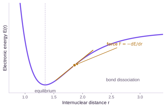
A worked bond curve: energy, force, and curvature
The Morse potential makes all three derivative levels visible without solving an electronic problem:
\[U(r)=D_e\left(1-e^{-a(r-r_e)}\right)^2-D_e.\]The parameters are the dissociation energy \(D_e>0\), equilibrium distance \(r_e\), and inverse length scale \(a>0\). The subtraction makes the separated-atom limit zero. Differentiating once gives
\[\frac{dU}{dr} =2D_ea\left(1-e^{-a(r-r_e)}\right)e^{-a(r-r_e)},\]and the radial force is
\[F(r)=-2D_ea\left(1-e^{-a(r-r_e)}\right)e^{-a(r-r_e)}.\]The signs pass three limiting checks. At \(r=r_e\), the parenthesis vanishes and \(F=0\). If \(r>r_e\), both factors in parentheses are positive, so \(F<0\) pulls the atoms together. As \(r\to\infty\), the exponential vanishes and so does the force. Compression gives \(r<r_e\), hence \(1-e^{-a(r-r_e)}<0\) and \(F>0\), pushing the atoms apart.
Take \(D_e=400\) kJ/mol, \(a=2\) Å\(^{-1}\), and stretch the bond by \(0.10\) Å. Then \(e^{-a(r-r_e)}=e^{-0.2}\approx0.819\), so
\[F\approx -2(400)(2)(1-0.819)(0.819) \approx-237\;\text{kJ mol}^{-1}\text{Å}^{-1}.\]The number is a restoring force, not an energy difference. Near equilibrium, set \(q=r-r_e\) and use \(e^{-aq}\approx1-aq\). Substitution gives
\[U(r)\approx-D_e+D_ea^2q^2 =-D_e+\frac{1}{2}kq^2, \qquad k=2D_ea^2.\]For the numerical parameters, \(k=3200\) kJ mol\(^{-1}\) Å\(^{-2}\). The local vibrational frequency is \(\omega=\sqrt{k/\mu}\) for reduced mass \(\mu\). The potential’s asymmetric dissociation tail disappears in this quadratic approximation, so a Hessian describes small vibrations but not bond breaking.
This gradient relation imposes a useful consistency condition on machine-learned force fields. A model that predicts a scalar energy and differentiates it produces a conservative force field by construction. A model that predicts forces directly can fit local vectors accurately while violating energy conservation unless the architecture or loss controls the curl. The right choice depends on whether long trajectories, energy conservation, or only local relaxation matters.
The curvature of the PES controls small motions around equilibrium. If \(\mathbf{R}_{*}\) is a local minimum, a second-order expansion gives
\[E_0(\mathbf{R}_{*}+\boldsymbol{\delta}) \approx E_0(\mathbf{R}_{*}) +\frac{1}{2}\boldsymbol{\delta}^{\top} \mathbf{K}\boldsymbol{\delta}, \qquad \mathbf{K}=\nabla_{\mathbf{R}}^2E_0(\mathbf{R}_{*}).\]The Hessian \(\mathbf{K}\) couples atomic displacements. After mass weighting and removal of rigid motions, its eigenvectors are normal modes and its eigenvalues determine squared vibrational frequencies. Energy, force, and curvature are therefore three derivative levels of one surface. A model trained only on energies may not learn accurate forces; one trained on energies and forces may still have poor vibrational spectra if its local curvature is wrong.
Wavefunctions, electron densities, orbitals, and bands
The exact wavefunction is too large for routine chemistry, so electronic-structure methods replace it with a tractable approximation. Molecular orbital theory expands one-electron orbitals in basis functions centered on atoms. Combining two atomic orbitals produces bonding and antibonding combinations: constructive interference can concentrate amplitude between nuclei, while destructive interference introduces a node. Filling these orbitals gives a compact qualitative account of covalent bonding.
The highest occupied molecular orbital (HOMO) and lowest unoccupied molecular orbital (LUMO) often indicate where electron removal and addition begin. Their energy difference is a useful descriptor, but it is not a universal measure of chemical stability or reactivity. Reaction barriers, solvent, spin, conformation, and orbital symmetry can dominate. In Kohn–Sham density functional theory (DFT), the orbital-energy difference is also not generally equal to the experimental fundamental gap because the exact functional has a derivative discontinuity and approximate functionals introduce additional error.
DFT avoids direct manipulation of the full many-electron wavefunction by using the electron density \(\rho(\mathbf{r})\) as its central variable. The Hohenberg–Kohn theorems establish that the ground-state density determines the external potential and that the correct density minimizes an energy functional (Hohenberg & Kohn, 1964). Kohn and Sham map the interacting problem to auxiliary one-electron equations with the same density (Kohn & Sham, 1965). The unknown exchange–correlation functional must still be approximated. Conventional Kohn–Sham calculations often scale roughly cubically with system size because they solve an orbital eigenproblem, though the actual scaling and prefactor depend on the algorithm, basis, accuracy, and system.
The Kohn–Sham equations make the approximation boundary explicit:
\[\left[ -\frac{1}{2}\nabla^2 +v_{\mathrm{ext}}(\mathbf{r}) +v_{\mathrm{H}}[\rho](\mathbf{r}) +v_{\mathrm{xc}}[\rho](\mathbf{r}) \right]\phi_i(\mathbf{r}) =\varepsilon_i\phi_i(\mathbf{r}).\]The external potential \(v_{\mathrm{ext}}\) comes from the nuclei, the Hartree potential \(v_{\mathrm{H}}\) is the classical electron repulsion, and the exchange–correlation potential \(v_{\mathrm{xc}}\) contains the unknown many-body remainder. The density reconstructed from occupied orbitals changes the potentials, so the equations are solved self-consistently. DFT is not “exact quantum mechanics made cheap”; its practical accuracy depends on the exchange–correlation approximation, basis, pseudopotentials, numerical settings, and the chemistry being studied.
In a crystal, periodicity changes the language from discrete molecular orbitals to bands. Bloch’s theorem labels electronic states by a wavevector in the reciprocal-space unit cell. A macroscopic number of closely spaced states forms energy bands. The highest occupied region is the valence band; low-lying empty states form the conduction band. Metals have partially filled bands or overlapping valence and conduction bands. Insulators have a gap too large for ordinary thermal excitation, while semiconductors have a gap that carriers can cross through temperature, light, or doping. The boundary is quantitative and context-dependent, not a separate kind of quantum mechanics.
Chemical forces are regimes of the same interaction
Chemists describe interactions as covalent, ionic, metallic, hydrogen-bonding, dipolar, or dispersive because these categories expose recurring mechanisms. They should not be mistaken for separate fundamental force laws. At the microscopic level, all arise from electrons and nuclei interacting electromagnetically under quantum mechanics.
Covalent bonding involves shared electron density and is strongly directional. Ionic bonding emphasizes electrostatic attraction after substantial charge transfer. Metallic bonding involves electrons delocalized across many atomic centers and connects naturally to partially filled bands. Real bonds can mix these characters; a single discrete label is often an approximation to a continuum.
Intermolecular interactions operate across molecular boundaries. A permanent dipole produces an orientation-dependent electrostatic interaction with another dipole. A hydrogen bond combines electrostatics, polarization, charge transfer, and dispersion in a directional geometry, often written as donor–H···acceptor. London dispersion arises from correlated fluctuations of electron density and exists even between nonpolar atoms. Its leading long-range contribution between two neutral fragments has the form
\[U_{\mathrm{disp}}(r)\approx-\frac{C_6}{r^6},\]where \(C_6\) depends on the fragments’ polarizabilities. The formula is asymptotic: it fails at short range, where electron-cloud overlap creates strong Pauli repulsion and many-body effects become relevant.
Energy-scale tables are useful only as rough orientation. A weak interaction repeated many times can dominate a free energy, while a strong bond may never break on the timescale of interest. Solvation can screen electrostatics, geometry can frustrate a hydrogen bond, and entropy can oppose an energetically favorable contact. The system-level outcome depends on populations, not one optimized structure.
Classical force fields turn these qualitative mechanisms into an explicit approximation to the PES. A common functional form is
\[U(\mathbf{R}) = \sum_{\text{bonds}} k_b(r-r_0)^2 +\sum_{\text{angles}} k_{\theta}(\theta-\theta_0)^2 +\sum_{\text{torsions}} V_n[1+\cos(n\phi-\delta)] +\sum_{i<j} \left[ 4\epsilon_{ij}\left( \frac{\sigma_{ij}^{12}}{r_{ij}^{12}} -\frac{\sigma_{ij}^{6}}{r_{ij}^{6}} \right) +\frac{q_iq_j}{4\pi\epsilon_0r_{ij}} \right].\]The first three sums describe bonded distortions; the final sum combines Lennard–Jones and fixed-charge electrostatic interactions. The decomposition is computationally convenient, not unique. Fixed charges omit explicit polarization, pairwise dispersion omits many-body dispersion, and a preset bond graph cannot describe bond breaking. Reactive force fields and ML potentials relax some of these assumptions, but every potential still inherits the support and accuracy of its reference data.
Statistical mechanics turns energies into populations
A molecular system at finite temperature does not occupy only its minimum-energy geometry. It explores an ensemble of microscopic states. In the canonical ensemble, the number of particles \(N\), volume \(V\), and temperature \(T\) are fixed while the system exchanges energy with a heat bath (Frenkel & Smit, 2002). If \(x\) denotes a full microscopic state with Hamiltonian \(\mathcal{H}(x)\), its equilibrium probability density is
\[p(x)=\frac{e^{-\beta \mathcal{H}(x)}}{Z}, \qquad Z=\int e^{-\beta \mathcal{H}(x)}\,dx, \qquad \beta=\frac{1}{k_{B}T}.\]The partition function \(Z\) normalizes the distribution. It also connects microscopic energies to the Helmholtz free energy,
\[A=-k_{B}T\log Z.\]For classical nuclei with momenta integrated out, the configurational distribution is proportional to \(e^{-\beta U(\mathbf{R})}\), where \(U\) is the potential energy. An energy difference \(\Delta U\) changes an equilibrium probability ratio exponentially:
\[\frac{p(x_2)}{p(x_1)}=e^{-\beta\Delta U}.\]At room temperature, \(k_{B}T\) is about \(2.5\) kJ/mol. A state only \(5\) kJ/mol higher in potential energy therefore receives roughly \(e^{-2}\approx0.14\) times the probability density of the lower state, before accounting for how much configuration-space volume surrounds either state.
From microscopic energies to basin populations
The probability of a macrostate is a sum over its microstates, so multiplicity competes directly with energy. Consider a discrete toy system in which basin \(A\) contains one microstate of energy \(0\) and basin \(B\) contains \(100\) microstates, each with energy \(5\) kJ/mol. At \(300\) K, using \(RT\approx2.49\) kJ/mol for molar energies, their partition-function contributions are
\[Z_A=1, \qquad Z_B=100\exp\!\left(-\frac{5}{2.49}\right) \approx13.4.\]Basin \(B\) is higher in potential energy at every one of its microstates, yet its equilibrium population is
\[P(B)=\frac{Z_B}{Z_A+Z_B} \approx\frac{13.4}{14.4} \approx0.93.\]Its larger volume wins. The same result can be written as a free-energy difference. The hundredfold multiplicity contributes an entropy difference \(\Delta S=R\log100\), so
\[\Delta G_{A\to B} =5\;\text{kJ/mol}-RT\log100 \approx5-11.5 =-6.5\;\text{kJ/mol}.\]Substituting into \(P(B)/P(A)=e^{-\Delta G/(RT)}\) gives \(e^{6.5/2.49}\approx13.6\), consistent with direct counting up to rounding. If the temperature approached zero, the entropy term \(T\Delta S\) would vanish and the lower-energy basin would dominate. This limiting check separates energetic preference from finite-temperature population.
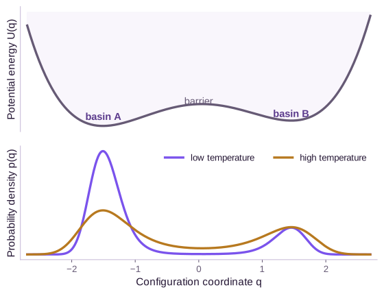
The last clause is where entropy enters. A broad basin can outweigh a narrow, deeper minimum because many microstates contribute to it. The figure below holds the energy landscape fixed while changing temperature. The low-temperature distribution concentrates near the deeper minimum. At higher temperature, the distribution spreads and the shallower basin gains population.
Entropy is a property of a probability distribution, not a synonym for visible disorder. For a classical continuous distribution,
\[S=-k_{B}\int p(x)\log p(x)\,dx,\]with the usual care about the reference measure for continuous entropy. Enthalpy is \(H=U+pV\), not simply an average potential energy. At constant temperature and pressure, the relevant potential is the Gibbs free energy
\[G=H-TS.\]The constant-pressure partition function gives the corresponding statistical definition of \(G\). By contrast, \(-k_{B}T\log Z\) for a canonical, fixed-volume partition function is the Helmholtz free energy. Keeping these ensembles distinct prevents a common but consequential notation error.
For two macrostates \(A\) and \(B\) at equilibrium, their Gibbs free-energy difference is related to their probability ratio by
\[\Delta G_{A\to B}=-k_{B}T\log\frac{P(B)}{P(A)}.\]This equation explains why free-energy prediction is harder than evaluating the energy of two optimized structures. Each probability integrates over an entire basin of solvent arrangements, conformations, protonation states, and other degrees of freedom. Endpoint energies alone omit that volume.
The conversion is also useful in reverse. A measured population ratio of \(P(B):P(A)=9:1\) at \(300\) K implies
\[\Delta G_{A\to B} =-RT\log9 \approx-(2.49)(2.20) \approx-5.5\;\text{kJ/mol}.\]A probability close to one does not require a large molar free-energy gap. Thermal energy is only a few kJ/mol, so errors that appear small beside a covalent bond energy can substantially distort conformer or binding populations.
The same integration defines a free-energy surface along a reduced coordinate. Let \(\xi(\mathbf{R})\) be a reaction coordinate such as a bond distance, torsion angle, or protein folding descriptor. Its equilibrium density is
\[p_{\xi}(s) = \frac{1}{Z_{R}} \int \delta\!\left(s-\xi(\mathbf{R})\right) e^{-\beta U(\mathbf{R})} \,d\mathbf{R},\]where \(Z_R\) normalizes the configurational distribution. The corresponding potential of mean force is
\[F(s)=-k_{B}T\log p_{\xi}(s)+C,\]with an arbitrary additive constant \(C\). This free-energy surface is not the potential energy evaluated at one representative structure. At each value of \(s\), it integrates over every unobserved coordinate. Changing the reaction coordinate changes that integration and can hide barriers that exist in the full space.
Dynamics decides which states can be reached
An equilibrium distribution says how much probability each region should have after complete equilibration. It does not say whether a simulation or experiment will reach that equilibrium. Molecular dynamics supplies time evolution.
For classical nuclei on a PES, Newton’s equations are
\[\frac{d\mathbf{R}_t}{dt}=\mathbf{V}_t, \qquad \mathbf{M}\frac{d\mathbf{V}_t}{dt}=-\nabla U(\mathbf{R}_t).\]Here \(\mathbf{M}\) is the diagonal mass matrix. These deterministic equations conserve total energy up to numerical integration error. To sample a canonical ensemble, Langevin dynamics adds friction and random collisions with an implicit heat bath:
\[d\mathbf{R}_t=\mathbf{V}_t\,dt,\] \[\mathbf{M}\,d\mathbf{V}_t = -\nabla U(\mathbf{R}_t)\,dt -\gamma\mathbf{M}\mathbf{V}_t\,dt +\sqrt{2\gamma k_{B}T\mathbf{M}}\,d\mathbf{W}_t.\]The friction coefficient \(\gamma\) removes kinetic energy, while the Wiener increment \(d\mathbf{W}_t\) injects fluctuations. Their amplitudes are linked by the fluctuation–dissipation relation, which makes the Boltzmann distribution stationary. Changing friction without changing noise generally changes the sampled temperature.
The stationary-distribution claim follows from density dynamics, not from the appearance of random noise alone. For the simpler overdamped Langevin equation
\[d\mathbf{R}_t = -\mu\nabla U(\mathbf{R}_t)\,dt +\sqrt{2\mu k_{B}T}\,d\mathbf{W}_t,\]the probability density obeys
\[\frac{\partial p_t}{\partial t} = \mu\nabla\cdot \left[p_t\nabla U+k_{B}T\nabla p_t\right].\]Substituting \(p_{\mathrm{eq}}(\mathbf{R})\propto e^{-\beta U(\mathbf{R})}\) makes the bracket vanish because \(k_{B}T\nabla p_{\mathrm{eq}}=-p_{\mathrm{eq}}\nabla U\). Drift pushes configurations downhill while diffusion spreads them uphill, and equilibrium is the exact balance. The Fokker–Planck equation article derives the general density evolution from both discretization and Itô calculus.
The PES organizes both conformational motion and chemical reactions. Local minima represent stable or metastable structures. A first-order saddle point has one downhill direction and often approximates a transition state between basins. For a nonlinear molecule in free space, the internal PES has roughly \(3N-6\) coordinates after removing global translation and rotation. Even a modest molecule therefore lives on a landscape that cannot be plotted directly; one-dimensional reaction coordinates are projections.
Thermodynamics and kinetics answer different questions. A negative reaction free energy \(\Delta G\) makes products more favorable at equilibrium. The activation free energy \(\Delta G^{\ddagger}\) controls how rapidly the system crosses the intervening bottleneck. Transition-state theory gives the approximate rate
\[k\approx\frac{k_{B}T}{h} e^{-\Delta G^{\ddagger}/(k_{B}T)},\]where \(h\) is Planck’s constant (Eyring, 1935). The exponential makes a small barrier error a large rate error. At \(300\) K, lowering a barrier by about \(5.7\) kJ/mol changes this exponential factor by roughly tenfold.
Barrier errors become clock errors
The prefactor at \(300\) K is approximately
\[\frac{k_{B}T}{h}\approx6.25\times10^{12}\;\text{s}^{-1}.\]For an activation free energy of \(75\) kJ/mol, transition-state theory predicts
\[k \approx (6.25\times10^{12}) \exp\!\left(-\frac{75}{2.49}\right) \approx0.52\;\text{s}^{-1}.\]Now suppose a learned potential overestimates only the transition region by \(4\) kJ/mol while fitting both minima exactly. The new rate is related to the old one without recomputing the prefactor:
\[\frac{k_{\mathrm{pred}}}{k_{\mathrm{true}}} =\exp\!\left(-\frac{4}{2.49}\right) \approx0.20.\]The predicted process is about five times too slow. An error of \(5.7\) kJ/mol gives a factor near \(0.10\), and an error of \(11.4\) kJ/mol gives a factor near \(0.01\). These are transition-region errors: a benchmark dominated by low-energy equilibrium structures may barely measure them.
Transition-state theory also has a boundary. It assumes near-equilibrium populations within the reactant basin, a dividing surface near the bottleneck, and negligible repeated recrossing. Strong dynamical recrossing, tunneling, solvent memory, or a poor reaction coordinate changes the prefactor or invalidates the reduction to one barrier. The exponential sensitivity remains a useful warning, but the formula is an approximation to dynamics, not its definition.
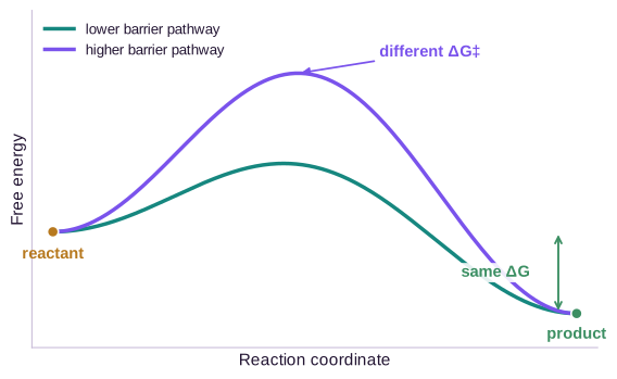
Two pathways can therefore have identical reactant and product free energies yet proceed at vastly different rates, as shown below. A catalyst changes the pathway and lowers the barrier; it does not need to change the equilibrium free-energy difference.
Metastability is the practical consequence. Diamond is thermodynamically less stable than graphite under ordinary conditions, yet the conversion is negligible because the required atomic rearrangement has a large barrier. Protein folding, ligand binding, diffusion through solids, and nucleation all exhibit related separation between local stability and transition time. A short trajectory can look stationary while remaining trapped in one basin.
Where molecular machine learning enters
The physical chain at the start now identifies several distinct ML problems. A property predictor maps a representation directly to an experimental observable. An electronic-structure surrogate predicts densities, orbitals, Hamiltonian matrices, or total energies. A machine-learned interatomic potential approximates \(U(\mathbf{R})\) and its gradient. A generative model approximates an equilibrium distribution or proposes structures that receive high probability under one. A dynamics model approximates trajectories, transition kernels, or rare-event pathways.
These tasks are not interchangeable. A model can predict equilibrium energies well and still produce poor long-time dynamics because small force errors accumulate or barriers are wrong. A generative model can match static conformer statistics without assigning physical time to its transitions. A graph model can predict a connectivity-dominated endpoint while failing on stereochemistry or crystal polymorphs. A periodic model can respect unit-cell translations while missing rare defects.
The strongest inductive bias is therefore a precise statement of the target. If the target is a scalar energy, impose the relevant invariances. If it is a force, impose equivariance and decide whether it must be an energy gradient. If it is an equilibrium population, model free energy rather than only minimum energy. If it is a rate, resolve the transition region rather than only the endpoints. Molecular ML becomes much less mysterious once each prediction is placed on the path from representation to energy, force, ensemble, and dynamics.
References
- Weininger, D. (1988). SMILES, a chemical language and information system. 1. Introduction to methodology and encoding rules. Journal of Chemical Information and Computer Sciences, 28(1), 31–36. ↩
- Heller, S. R., McNaught, A., Pletnev, I., Stein, S. & Tchekhovskoi, D. (2015). InChI, the IUPAC International Chemical Identifier. Journal of Cheminformatics, 7, 23. ↩
- Bronstein, M. M., Bruna, J., Cohen, T. & Veličković, P. (2021). Geometric deep learning: Grids, groups, graphs, geodesics, and gauges. arXiv:2104.13478. ↩
- Born, M. & Oppenheimer, R. (1927). Zur Quantentheorie der Molekeln. Annalen der Physik, 389(20), 457–484. ↩
- Szabo, A. & Ostlund, N. S. (1996). Modern Quantum Chemistry: Introduction to Advanced Electronic Structure Theory. Dover Publications. ↩
- Hohenberg, P. & Kohn, W. (1964). Inhomogeneous electron gas. Physical Review, 136(3B), B864–B871. ↩
- Kohn, W. & Sham, L. J. (1965). Self-consistent equations including exchange and correlation effects. Physical Review, 140(4A), A1133–A1138. ↩
- Frenkel, D. & Smit, B. (2002). Understanding Molecular Simulation: From Algorithms to Applications (2nd ed.). Academic Press. ↩
- Eyring, H. (1935). The activated complex in chemical reactions. The Journal of Chemical Physics, 3(2), 107–115. ↩