What Does a Molecular-Dynamics Program Actually Store and Update?

Molecular dynamics is a loop over arrays. Positions enter a potential-energy function, differentiation produces forces, an integrator updates positions and momenta, and selected states become a trajectory. The apparent complexity of an MD package comes from making this loop fast, physical, and difficult to misuse.

This chapter builds that mental model with two atoms. The example is small enough to inspect line by line, but it uses the same JAX operations and the same kinds of state that later chapters use for hundreds of atoms.

The state is more than a set of coordinates

For \(N\) atoms, the position array has shape \(N\times3\). Row \(i\) stores the Cartesian position \(\mathbf{r}_i=(x_i,y_i,z_i)\). An MD state usually also contains momenta \(\mathbf{p}_i\), masses \(m_i\), atomic numbers \(Z_i\), and a simulation cell \(\mathbf{H}\):

Here \(\mathbf{R}\) and \(\mathbf{P}\) are \(N\times3\) arrays. The cell \(\mathbf{H}\) is a \(3\times3\) matrix whose rows or columns, depending on the library convention, describe the box vectors. The ellipsis can contain a step counter, thermostat variables, cell momentum, neighbor data, or cached potential outputs.

Positions alone are not a complete dynamical state. Two systems with identical positions and opposite momenta immediately move in opposite directions. Atomic numbers and masses also play different roles: the potential generally uses chemical identity, while Newton’s equation uses mass to convert force into acceleration.

Units are part of this state contract. In the kUPS examples, positions enter through ASE in ångström, masses use atomic mass units, energies use electron volts, and user-facing timesteps are specified in femtoseconds. kUPS converts these values into its internally consistent representation. A bare array does not carry a unit label, so mixing conventions can produce a numerically smooth but physically meaningless trajectory.

Energy becomes force through a gradient

An interatomic potential maps all atomic positions to one scalar:

The force on atom \(i\) is the negative derivative of that scalar with respect to the atom’s position:

The minus sign points the force downhill on the energy surface. Because the input has shape \(N\times3\), the gradient and force arrays have that same shape.

For the two-atom example, let \(r=\lVert\mathbf{r}_2-\mathbf{r}_1\rVert\) and use a harmonic bond,

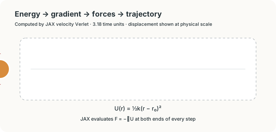
The equilibrium distance is \(r_0=1\), the spring constant is \(k=2\), and the initial distance is \(1.2\) in dimensionless units. The extension is therefore \(0.2\), giving an energy of \(0.04\) and a force magnitude of \(0.4\).

from functools import partial
from pathlib import Path
import os

repo_root = Path.cwd()
if not (repo_root / "configs").exists():
    repo_root = repo_root.parent
os.chdir(repo_root)
os.environ.setdefault("JAX_PLATFORMS", "cpu")

from ase import Atoms
import jax
import jax.numpy as jnp
from kups.application.md.data import MdParameters, md_state_from_ase

from kups_md_tutorials.jax_reference import (
    ParticleState,
    forces_from_energy,
    harmonic_pair_energy,
    kinetic_energy,
    simulate_velocity_verlet,
)

positions = jnp.array([[-0.60, 0.0, 0.0], [0.60, 0.0, 0.0]])
energy_fn = partial(
    harmonic_pair_energy,
    spring_constant=2.0,
    equilibrium_distance=1.0,
)
energy = energy_fn(positions)
forces = forces_from_energy(energy_fn, positions)

print(f"positions shape: {positions.shape}")
print(f"potential energy: {float(energy):.4f}")
print("forces on atoms:")
print(forces)
print(f"net force: {jnp.sum(forces, axis=0)}")

positions shape: (2, 3)
potential energy: 0.0400
forces on atoms:
[[ 0.4000001 -0.        -0.       ]
 [-0.4000001 -0.        -0.       ]]
net force: [0. 0. 0.]

The two force vectors are equal and opposite. Their sum is zero because translating both atoms by the same amount does not change their separation or the energy. This simple check catches sign, indexing, and broadcasting errors before a trajectory hides them among many updates.

JAX performs the derivative in forces_from_energy with jax.grad. This is automatic differentiation, not a finite-difference approximation. The energy function remains the primary object; JAX constructs the derivative program needed by the integrator.

An integrator turns one state into the next

Newton’s equations describe continuous time,

A computer cannot apply an infinitesimal change. An integrator chooses a finite timestep \(\Delta t\) and constructs a discrete map

The sequence \(X_0,X_1,\ldots,X_M\) is a trajectory. It approximates the continuous solution at specific times. It is not the exact motion with some frames omitted.

The reference code represents the state with three JAX arrays and repeatedly applies velocity Verlet. jax.lax.scan carries the new state into the next step and stacks the recorded states into trajectory arrays.

initial_state = ParticleState(
    positions=positions,
    momenta=jnp.zeros_like(positions),
    masses=jnp.ones(2),
)
final_state, trajectory = simulate_velocity_verlet(
    energy_fn, initial_state, time_step=0.02, num_steps=400
)
total_energy = jax.vmap(energy_fn)(trajectory.positions) + jax.vmap(
    kinetic_energy
)(trajectory)
relative_error = (total_energy - total_energy[0]) / total_energy[0]

print(f"trajectory positions: {trajectory.positions.shape}")
print(f"largest relative energy excursion: {float(jnp.max(jnp.abs(relative_error))):.3e}")
print(f"final separation: {float(jnp.linalg.norm(final_state.positions[1] - final_state.positions[0])):.3f}")

trajectory positions: (400, 2, 3)
largest relative energy excursion: 3.995e-04
final separation: 0.809

The result has shape (400, 2, 3): 400 stored states, two atoms, and three coordinates. The maximum relative energy excursion is about \(4.0\times10^{-4}\) for this timestep. A small bounded excursion is expected from velocity Verlet; it does not mean the discrete trajectory is exact. Post 02 opens the step itself and shows how the error changes with timestep and integration scheme.

An MD run often performs many steps between stored frames. If the block size is ten, the engine may update the state ten times and save only the tenth state. The trajectory file then has fewer frames than integration steps. This distinction becomes essential when interpreting time axes, correlations, and storage cost.

JAX changes how the loop is expressed

Ordinary Python code often mutates arrays inside a for loop. JAX works best when a step is a pure function: the old state enters and a new state leaves. That functional form enables several transformations used throughout the series:

• jax.grad turns a scalar energy program into a force calculation;
• jax.jit compiles a state update for the selected device and array shapes;
• jax.lax.scan expresses a repeated update without a Python dispatch per step;
• jax.vmap applies the same observable or model across frames or replicas;
• explicit PRNG keys make stochastic updates reproducible and composable.

These operations do not change the physics. They change how the computation is staged, differentiated, compiled, and parallelized. A correct JAX program must still use correct forces, units, boundaries, and update equations.

Periodic boundaries make the cell active

Bulk simulations use a finite box as a repeating tile. An atom leaving one side re-enters through the opposite side, and an atom near the left face can be a close neighbor of an atom near the right face.

The potential must therefore measure displacement using the selected periodic cell rather than raw Cartesian subtraction. The integrator must also decide whether to store wrapped positions inside the primary cell or an unwrapped path that records boundary crossings. Both representations can describe the same physical motion, but they support different analyses.

Periodic boundaries do not make a small system identical to an infinite one. The box length limits meaningful pair distances, changes which fluctuations fit inside the cell, and can couple an atom to its own periodic images. Later chapters make these finite-size limits explicit when computing radial distribution functions and free energies.

kUPS gives the arrays a production structure

The minimal ParticleState is useful because every operation is visible. A production engine must also represent multiple chemical species, one or more systems, cell geometry, particle-to-system indices, boundary flows, thermostat/barostat parameters, potential caches, logging, and recovery from invalid updates.

kUPS stores these pieces in structured JAX PyTrees. A PyTree is a nested Python object whose numerical leaves are arrays. JAX transformations can operate on the leaves while kUPS preserves their physical roles.

The next cell constructs an ASE system and passes it through the public kUPS state adapter. This is a real kUPS object, not a dictionary made to resemble one.

atoms = Atoms(
    "Ar2",
    positions=[[0.0, 0.0, 0.0], [4.0, 0.0, 0.0]],
    cell=[12.0, 12.0, 12.0],
    pbc=True,
)
md = MdParameters(
    temperature=100.0,
    time_step=1.0,
    friction_coefficient=0.0,
    thermostat_time_constant=100.0,
    target_pressure=0.0,
    pressure_coupling_time=1.0e10,
    compressibility=4.5e-10,
    minimum_scale_factor=1.0,
    integrator="verlet",
    initialize_momenta=True,
)
particles, systems = md_state_from_ase(atoms, md, key=jax.random.key(7))

print(f"positions: {particles.data.positions.shape}")
print(f"momenta: {particles.data.momenta.shape}")
print(f"masses: {particles.data.masses.shape}")
print(f"cell parameters: {systems.data.cell.frame.tril.shape}")
print(f"JAX leaves in state: {len(jax.tree.leaves((particles, systems)))}")

positions: (2, 3)
momenta: (2, 3)
masses: (2,)
cell parameters: (1, 6)
JAX leaves in state: 14

The particle table contains the same position, momentum, and mass arrays used by the minimal example. The system table adds the periodic cell and integrator parameters. The full state contains fourteen numerical leaves for this tiny case because kUPS also tracks indices, gradients, cell data, and system-level quantities.

A kUPS MD calculation can be read as four objects:

1. State: the current particle and system data.
2. Potential: a function that returns energy and the derivatives required by dynamics.
3. Propagator: a composable state update such as velocity Verlet, a thermostat, or a barostat.
4. Logger: a rule for selecting and writing frames and observables.

The later notebooks will keep this mapping visible. They first implement the central operation with small JAX arrays, then show the corresponding kUPS potential or propagator, and finally run the library path that writes the recorded evidence.

A trajectory is not an ensemble or an observable

A trajectory is an ordered sequence of states. An ensemble is a probability distribution over states under specified constraints, such as fixed particle number, volume, and energy. An observable is a quantity estimated from states, such as temperature, pressure, a radial distribution function, or a velocity correlation.

One long trajectory may provide samples from an ensemble, but only after the initial transient has decayed and only to the extent that stored frames contain independent information. Saving ten times as many highly correlated frames does not create ten times as much evidence. Posts 04–08 develop these distinctions using real kUPS trajectories.

Check your understanding

Before running the code, predict what happens if both atomic masses are doubled while the potential and initial positions remain fixed.

The energy and force are unchanged because neither depends on mass in this example. The acceleration is halved because \(\mathbf{a}=\mathbf{F}/m\), so the bond oscillates more slowly. Changing the spring constant instead changes both the force and the oscillation rate.

You can test the prediction by replacing jnp.ones(2) with 2 * jnp.ones(2) in the trajectory cell. The final separation at a fixed step count changes, but the opposite-force and zero-net-force checks still hold.

Post 01 now has a narrower job: construct a physically controlled initial state for many atoms. Post 02 then opens the velocity-Verlet map and connects its JAX implementation to the kUPS propagator.

git clone https://github.com/sungsoo-ahn/kups-md-tutorials
cd kups-md-tutorials
uv sync --locked

uv run pytest tests/test_jax_reference.py tests/test_foundation_visuals.py
uv run kups-tutorial verify-notebooks --posts 00 --output-dir notebook-runs
uv run kups-tutorial export-notebook-cells \
  --executed-notebooks-dir notebook-runs \
  --site-root ../sungsoo-ahn.github.io --posts 00 --check