Initialization chooses the first probability distribution in an MD experiment. It is not housekeeping before the “real” simulation. A cell that is too dense changes every periodic distance. A velocity draw with net drift moves the whole box. A minimization or warmup changes which configurations can appear in the measured trajectory.
This lesson constructs an argon crystal, implements its thermal momentum draw in JAX, removes rigid translation, and then performs the same state construction through kUPS. The important question is not whether an initialization function returns without error. It is: what distribution produced the first measured frame?
- which parts of an atomic state must be fixed before momenta are sampled;
- why a target temperature sets a distribution rather than an exact finite value;
- how the Maxwell–Boltzmann draw and center-of-mass correction become JAX code;
- what
md_state_from_aseadds when it constructs the real kUPS state; - why a valid initial state is not yet an equilibrated sample.
Prerequisites: atomic positions, momenta, masses, cells, JAX arrays, and explicit random keys from the foundations lesson.
First choose atoms, coordinates, and a periodic cell
An MD state needs atomic numbers \(\mathbf{z}\), positions \(\mathbf{R}\), momenta \(\mathbf{P}\), masses \(\mathbf{m}\), and a cell \(\mathbf{H}\). We must choose the first four deterministic ingredients before sampling \(\mathbf{P}\):
- the chemical identities and masses;
- the arrangement of atoms;
- the cell vectors;
- which directions are periodic.
The example is face-centered-cubic argon. Its number density \(\rho\) fixes the cell volume:
\[V = \det(\mathbf{H}) = \frac{N}{\rho}.\]Here \(N\) is the atom count, \(V\) is measured in cubic ångström, and \(\rho=0.0213\ \mathrm{atoms\,\mathring{A}^{-3}}\). The smoke calculation uses 32 atoms; the full state uses 500. Density is a physical input: changing it changes periodic distances, pressure, coordination, and the environments seen by a learned potential.
Temperature sets a momentum variance
For a classical atom \(i\) of mass \(m_i\), one Cartesian momentum component at temperature \(T\) follows
\[p_{i,\alpha} \sim \mathcal{N}\!\left(0,\,m_i k_B T\right),\]where \(\alpha\in\{x,y,z\}\) and \(k_B\) is Boltzmann’s constant. Heavy atoms therefore have wider momentum distributions. Their velocity distribution is narrower because \(v_{i,\alpha}=p_{i,\alpha}/m_i\).
For one sampled state, kinetic energy is
\[K(\mathbf{P}) = \sum_{i=1}^{N}\sum_{\alpha=1}^{3} \frac{p_{i,\alpha}^{2}}{2m_i}.\]If \(f\) independent velocity degrees of freedom remain, the instantaneous kinetic temperature is defined by
\[T_{\mathrm{inst}} = \frac{2K}{f k_B}.\]This is an estimator computed from one random draw. It need not equal the target \(T\). Forcing exact agreement by rescaling all momenta imposes another constraint on \(K\); it creates a different finite-state distribution and must be reported.
The draw is three JAX operations
The setup below only selects the repository and imports JAX and the kUPS workflow. It begins collapsed because none of those lines defines the algorithm.
Python
from pathlib import Path
import os

repo_root = Path.cwd()
if not (repo_root / "configs").exists():
    repo_root = repo_root.parent
os.chdir(repo_root)
os.environ.setdefault("JAX_PLATFORMS", "cpu")

import jax
from jax import Array
import jax.numpy as jnp
from IPython.display import Image, display
from kups_md_tutorials.config import load_tutorial_spec
from kups_md_tutorials.initialization import (
    load_kups_initialization_evidence,
    write_initialization_outputs,
)
The open cell implements the complete reference operation. First it draws standard normal values. Then it multiplies each atom’s row by \(\sqrt{m_i k_B T}\). Finally it subtracts rigid translation and measures the remaining kinetic temperature.
Python
BOLTZMANN_EV_PER_K = 8.617333262145e-5

def sample_maxwell_boltzmann_momenta(
    key: Array,
    masses: Array,
    temperature_k: float,
) -> Array:
    """Draw three momentum components per atom in ASE-compatible units."""

    standard_normal = jax.random.normal(key, (masses.shape[0], 3))
    component_scale = jnp.sqrt(
        masses[:, None] * BOLTZMANN_EV_PER_K * temperature_k
    )
    return component_scale * standard_normal


def remove_center_of_mass_momentum(momenta: Array, masses: Array) -> Array:
    """Remove the rigid translation without changing relative velocities."""

    center_of_mass_velocity = jnp.sum(momenta, axis=0) / jnp.sum(masses)
    return momenta - masses[:, None] * center_of_mass_velocity


def instantaneous_temperature(
    momenta: Array,
    masses: Array,
    *,
    removed_center_of_mass: bool = True,
) -> Array:
    """Convert kinetic energy to temperature for the stated degrees of freedom."""

    kinetic = 0.5 * jnp.sum(momenta**2 / masses[:, None])
    degrees_of_freedom = momenta.size - (3 if removed_center_of_mass else 0)
    return 2.0 * kinetic / (degrees_of_freedom * BOLTZMANN_EV_PER_K)


masses = jnp.full((32,), 39.948)
raw = sample_maxwell_boltzmann_momenta(jax.random.PRNGKey(7), masses, 94.4)
stationary = remove_center_of_mass_momentum(raw, masses)
mean_velocity = jnp.sum(stationary, axis=0) / jnp.sum(masses)
print(f"realized temperature={instantaneous_temperature(stationary, masses):.2f} K")
print(f"box speed after removal={jnp.linalg.norm(mean_velocity):.3e}")realized temperature=85.83 K
box speed after removal=2.389e-10
jax.random.PRNGKey(7) makes randomness an explicit input. Reusing that key repeats the draw; splitting it creates independent keys. This functional randomness matters under jit, vmap, and parallel replica generation, because there is no hidden global generator for a compiled function to advance.
The 32-atom result misses 94.4 K by a visible amount. That is the expected finite-sample fluctuation of \(3N-3=93\) quadratic degrees of freedom, not an initialization failure. More atoms narrow this fluctuation, but they do not turn a random variable into a deterministic number.
Remove box translation, not thermal motion
A raw draw usually gives the box a nonzero center-of-mass velocity:
\[\mathbf{V}_{\mathrm{COM}} =\frac{\sum_i \mathbf{p}_i}{\sum_i m_i}.\]Subtracting the corresponding momentum from every atom gives
\[\mathbf{p}'_i = \mathbf{p}_i-m_i\mathbf{V}_{\mathrm{COM}}.\]The corrected total momentum is exactly zero in exact arithmetic:
\[\sum_i \mathbf{p}'_i =\sum_i \mathbf{p}_i -\mathbf{V}_{\mathrm{COM}}\sum_i m_i =\mathbf{0}.\]This removes three degrees of freedom, so the temperature denominator becomes \(f=3N-3\). It does not set individual velocities to zero. The atoms retain relative thermal motion, which is what drives internal dynamics.
Removing rotation is a different operation and is usually inappropriate for a periodic bulk crystal. Likewise, preserving temperature after drift removal rescales the remaining momenta. Each transformation changes the distribution and should be an explicit choice.
kUPS constructs the production state
The reference JAX code makes the mathematics visible. The actual tutorial run uses the public kUPS adapter. It reads the ASE structure, builds kUPS particle and cell PyTrees, draws momenta from a JAX key, and removes center-of-mass motion.
Python
smoke = load_tutorial_spec("01", "smoke")
result_dir = write_initialization_outputs(
    smoke, output_root=Path("runs/notebook-post-01")
)
evidence = load_kups_initialization_evidence(
    result_dir / "kups_initialization_summary.json"
)
print(evidence.entry_point)
print(f"device={evidence.observed_devices[0]}")
print(f"positions={evidence.position_shape}, momenta={evidence.momentum_shape}")
print(f"kUPS draw: {evidence.instantaneous_temperature_k:.2f} K")
print(f"center-of-mass speed={evidence.center_of_mass_speed:.3e}")
print(f"momenta sha256={evidence.momenta_sha256[:16]}...")kups.application.md.data.md_state_from_ase
device=cpu:cpu
positions=(32, 3), momenta=(32, 3)
kUPS draw: 72.11 K
center-of-mass speed=5.434e-10
momenta sha256=e66926230d66840d...
The cell executes kups.application.md.data.md_state_from_ase; it does not load a committed summary and call that execution. The output reports the observed JAX device, array shapes, realized temperature, residual box speed, and a digest of the returned momenta.
The full 500-atom run returns position and momentum arrays of shape (500, 3). Its realized kinetic temperature is 95.37 K for a 94.4 K target, and its center-of-mass speed is \(3.32\times10^{-10}\) in the recorded internal velocity units. These values establish a finite, stationary state. They do not establish equilibrium.
Look at the state before propagating it
The next figure reads the positions, momenta, masses, and cell serialized from the full kUPS return value. The left panel selects one layer so velocity arrows remain legible. Their lengths are scaled for display and do not represent an elapsed trajectory. The right panel uses all 1,500 Cartesian momentum components.
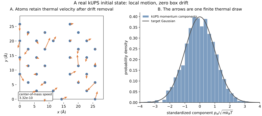
The absence of a preferred arrow direction is the atom-level meaning of the small center-of-mass speed. The approximate Gaussian is a distribution-level check. Neither plot can tell us whether the positions are equilibrated for the chosen potential and temperature.
Initialization and equilibration answer different questions
A syntactically valid state can still be physically poor. The crystal may be too dense, contain overlapping atoms, or sit far from the target potential’s typical energy range. Thermal momenta do not repair those problems.
Common follow-up operations change the state in distinct ways:
These distinctions are standard in molecular-simulation methodology (Frenkel & Smit, 2001; Tuckerman, 2010).
| Operation | What it changes | What it does not prove |
|---|---|---|
| energy minimization | moves positions toward a nearby local minimum | thermal sampling |
| velocity rescaling | fixes total kinetic energy | correct configurational distribution |
| thermostat warmup | evolves momenta and positions under a temperature controller | independence from the starting structure |
| pressure equilibration | evolves the cell and density | unbiased production statistics |
The production trajectory should begin only after the relevant transient has been diagnosed and the discarded interval has been declared. For a controlled integrator comparison, reuse the same initialized state. For uncertainty estimation, change the key and run independent replicas. Those are different experimental designs.
Check your understanding
Suppose every atom receives the same added velocity \(\mathbf{u}\) before the center-of-mass correction.
- Predict the corrected momenta without running code.
- Does the correction recover the original relative velocities for atoms of different masses?
- Change the notebook from 32 to 3,200 atoms. Predict what happens to the spread of \(T_{\mathrm{inst}}\) across independent keys, then test it with
jax.vmap.
The first two answers follow directly from \(\mathbf{p}'_i=\mathbf{p}_i-m_i\mathbf{V}_{\mathrm{COM}}\). The third turns the phrase “finite-sample fluctuation” into a measurable scaling experiment.
What to carry into the trajectory
An initialization record must bind coordinates, cell, identities, masses, momentum rule, random key, constraints, and implementation. In this run, the state digest changes if any of those inputs or operations changes. That makes the starting point reproducible.
It is still only a starting point. Post 02 now asks how forces turn this state into a discrete trajectory, while later chapters decide which transient frames to discard and which observables to trust.
Reproducibility record and complete diagnostic dashboard
Run and verify the CPU profile from a locked environment:
git clone https://github.com/sungsoo-ahn/kups-md-tutorials
cd kups-md-tutorials
uv sync --locked

uv run kups-tutorial run 01 --profile smoke
uv run kups-tutorial verify 01 --profile smoke
uv run kups-tutorial verify-notebooks --posts 01 --output-dir notebook-runs
uv run kups-tutorial export-notebook-cells \
  --executed-notebooks-dir notebook-runs \
  --site-root ../sungsoo-ahn.github.io --posts 01 --check
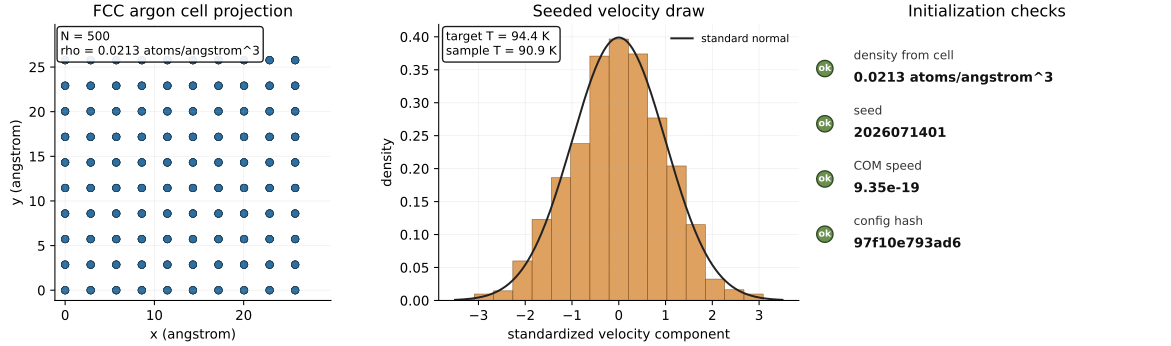
The complete audit retains the FCC projection, the earlier ASE control, and the kUPS evidence panel:
Source and evidence: