ProteinMPNN: Inverse Folding and Sequence Design
This is Lecture 6 of the Protein & Artificial Intelligence course (Spring 2026), co-taught by Prof. Sungsoo Ahn and Prof. Homin Kim at KAIST Graduate School of AI. The lecture builds on concepts from Lecture 4 (AlphaFold) and Lecture 5 (RFDiffusion). Familiarity with graph neural networks (Preliminary Lecture 4) and generative models (Preliminary Lecture 5) is assumed throughout.
Introduction
Suppose you have just used RFDiffusion to generate a protein backbone—a custom binder for a therapeutic target, or an enzyme scaffold with catalytic residues placed at precise coordinates. The backbone exists as a set of three-dimensional coordinates, but proteins are not manufactured from coordinates. They are built from sequences of amino acids, translated from genetic code by ribosomes in living cells. To make your designed protein in the laboratory, you need a sequence of amino acids that will reliably fold into that backbone.
Finding such a sequence is the inverse folding problem, and ProteinMPNN1 is the tool that solves it. Given a backbone structure, ProteinMPNN outputs a probability distribution over amino acid sequences conditioned on that structure. You can then sample from this distribution to obtain diverse candidate sequences, each predicted to fold into the target backbone.
This lecture covers the full ProteinMPNN system: how it represents protein structure as a graph, how it encodes that graph into rich per-residue features, how it generates sequences one amino acid at a time, and how it integrates into the RFDiffusion \(\to\) ProteinMPNN \(\to\) AlphaFold design pipeline that has become the standard workflow in computational protein design.
Roadmap
| Section | Topic | Why It Is Needed |
|---|---|---|
| 1 | The Inverse Folding Problem | Defines the task ProteinMPNN solves and explains why multiple sequences can fold into the same structure |
| 2 | Graph Construction | Translates raw backbone coordinates into a data structure that neural networks can process |
| 3 | Edge Features | Provides a rich geometric vocabulary beyond simple distances |
| 4 | The Structure Encoder | Propagates local geometric information across the protein through message passing |
| 5 | Autoregressive Decoding | Generates amino acids one at a time, capturing inter-residue dependencies |
| 6 | Training | Describes the loss function, random-order training, and data augmentation |
| 7 | Advanced Features | Handles practical constraints: fixed positions, symmetry, and tied sequences |
| 8 | The Design Pipeline | Connects RFDiffusion, ProteinMPNN, and AlphaFold into an end-to-end workflow |
| 9 | Design Principles and Alternatives | Summarizes what makes ProteinMPNN work and compares it with other inverse folding methods |
| 10 | Exercises | Practice problems to consolidate understanding |
1. The Inverse Folding Problem
Forward Folding vs. Inverse Folding
flowchart LR
    subgraph Forward["Forward Folding"]
        SEQ1["Amino Acid\nSequence"] -->|"AlphaFold\nESMFold"| STR1["3D\nStructure"]
    end

    subgraph Inverse["Inverse Folding"]
        STR2["3D\nStructure"] -->|"ProteinMPNN"| SEQ2A["Sequence 1"]
        STR2 -->|"ProteinMPNN"| SEQ2B["Sequence 2"]
        STR2 -->|"ProteinMPNN"| SEQ2C["Sequence 3"]
    end

    style Forward fill:#e8f4fd,stroke:#2196F3
    style Inverse fill:#e8f5e9,stroke:#4CAF50
In Lecture 4, we studied forward folding: given a sequence of amino acids, predict the three-dimensional structure. AlphaFold solves this problem with near-experimental accuracy. The forward direction mirrors what happens in biology—DNA encodes a protein sequence, and physics determines how that sequence folds.
Inverse folding goes the other way. Given a target backbone structure, find amino acid sequences that will fold into it. If AlphaFold is a compiler that turns source code into an executable, ProteinMPNN is a decompiler that recovers source code from the executable.
Forward folding:   MKFLILLFNILCLFPVLAADNH...  -->  3D Structure
                   (AlphaFold, ESMFold)

Inverse folding:   3D Structure  -->  MKFLILLFNILCLFPVLAADNH...
                                  -->  MKYLILIFNLLCLFPVLAADNH...
                                  -->  MRFLILIFNILCLYPVLAADNQ...
                   (ProteinMPNN)       (multiple valid sequences)
Notice a fundamental asymmetry in this diagram. Forward folding typically produces a single dominant structure from a given sequence2. Inverse folding produces many valid sequences for a single structure. This many-to-one mapping is central to understanding why inverse folding is both tractable and useful.
The Many-to-One Mapping
Why can multiple sequences fold into the same structure? The answer lies in the physics of protein folding and the lessons of molecular evolution.
Consider hemoglobin. Human hemoglobin and fish hemoglobin perform the same oxygen-carrying function and adopt remarkably similar three-dimensional structures, yet their sequences can differ by more than 50%. Or consider the immunoglobulin fold—this basic structural motif appears in thousands of different antibody sequences across the immune system, each with unique binding specificity encoded in variable loops but sharing the same underlying architecture.
This sequence tolerance exists because not every amino acid position contributes equally to structural stability. Some positions sit in the hydrophobic core, where the main requirement is “something nonpolar”—valine, leucine, or isoleucine might all work equally well. Other positions face the solvent and can tolerate almost any hydrophilic residue. Only a subset of positions—those involved in specific hydrogen bonds, salt bridges, or tight packing interactions—are tightly constrained.
Structural biologists quantify this tolerance with sequence identity thresholds. Proteins with as little as 20–30% sequence identity often share the same fold. This means roughly 70–80% of positions can vary without disrupting the overall architecture. For inverse folding, this redundancy is a blessing: there is a vast space of valid sequences for any given structure, making the search problem tractable.
ProteinMPNN captures this diversity by learning a conditional probability distribution:
\[P(\mathbf{s} \mid \mathcal{X})\]where \(\mathbf{s} = (s_1, s_2, \dots, s_L)\) is a sequence of \(L\) amino acids and \(\mathcal{X}\) denotes the backbone structure (the set of backbone atom coordinates). Rather than outputting a single “best” sequence, the model provides probabilities for each amino acid at each position, allowing us to sample diverse sequences that are all predicted to fold correctly.
Why Inverse Folding Matters
Inverse folding has become one of the most practically important tools in computational protein design for four reasons.
Completing the design pipeline. Backbone generation methods like RFDiffusion (Lecture 5) produce three-dimensional coordinates, but these are not directly manufacturable. Inverse folding provides the missing link, converting geometric designs into genetic sequences that can be ordered as synthetic DNA and expressed in cells.
Sequence optimization. Sometimes you already have a protein that works but could be better—perhaps it expresses poorly in your production system, or it aggregates during purification. Inverse folding can suggest alternative sequences that maintain the same structure while potentially improving biochemical properties like solubility or thermostability.
Exploring sequence space. For a given backbone, inverse folding can generate hundreds of diverse sequences. This is invaluable for experimental screening: you test many variants simultaneously and identify sequences with favorable properties that no single computational method would have predicted.
Understanding evolution. By analyzing which sequence features ProteinMPNN considers important for a given structure, we gain insight into the molecular determinants of protein folding—essentially reverse-engineering nature’s design rules.
2. Graph Construction: Proteins as k-Nearest Neighbor Graphs
flowchart LR
    BACKBONE["Backbone\nCoordinates\n(N, Cα, C, O)"] --> DIST["Compute Cα\nDistances"]
    DIST --> KNN["k-Nearest\nNeighbors\n(k = 30)"]
    KNN --> GRAPH["Protein Graph\nL nodes\n30·L edges"]

    style BACKBONE fill:#e8f4fd,stroke:#2196F3
    style GRAPH fill:#e8f5e9,stroke:#4CAF50
The first step in ProteinMPNN’s pipeline is converting a protein backbone into a graph. This is where the geometric nature of the problem gets translated into a form that a neural network can process.
Why Graphs?
Proteins have an obvious graph-like quality. Each residue is a discrete unit (a natural node), and the spatial relationships between residues define natural edges. Unlike images, which live on regular grids, protein structures are irregular: residues that are far apart in the amino acid sequence may be close together in three-dimensional space because the chain folds back on itself. Graph neural networks handle this irregularity natively.
Building the k-NN Graph
For each residue, ProteinMPNN finds its \(k\) nearest neighbors based on the Euclidean distance between their alpha-carbon (\(\text{C}_\alpha\)) atoms. A typical choice is \(k = 30\), meaning each residue connects to its 30 closest spatial neighbors.
Why \(\text{C}_\alpha\) distances? The alpha-carbon sits at the geometric center of each amino acid’s backbone, making it a stable reference point for the overall residue position. While more elaborate distance measures are possible (e.g., using multiple backbone atoms), \(\text{C}_\alpha\) distances are effective and computationally cheap.
import torch
import torch.nn as nn

def build_knn_graph(ca_coords, k=30, exclude_self=True):
    """
    Build a k-nearest neighbor graph from alpha-carbon coordinates.

    Args:
        ca_coords: [L, 3] tensor of C-alpha positions for L residues.
        k: Number of neighbors per residue.
        exclude_self: If True, a residue cannot be its own neighbor.

    Returns:
        edge_index: [2, E] tensor where E = L * k. Row 0 is source, row 1 is destination.
        edge_dist:  [E] tensor of Euclidean distances for each edge.
    """
    L = ca_coords.shape[0]

    # Pairwise distance matrix: dist[i, j] = ||CA_i - CA_j||
    diff = ca_coords.unsqueeze(0) - ca_coords.unsqueeze(1)  # [L, L, 3]
    dist = diff.norm(dim=-1)  # [L, L]

    if exclude_self:
        dist.fill_diagonal_(float('inf'))  # prevent self-loops

    # For each residue, select the k nearest neighbors
    _, neighbors = dist.topk(k, dim=-1, largest=False)  # [L, k]

    # Flatten into edge list
    src = torch.arange(L).unsqueeze(-1).expand(-1, k).reshape(-1)
    dst = neighbors.reshape(-1)
    edge_index = torch.stack([src, dst])  # [2, L*k]

    edge_dist = dist[src, dst]  # [L*k]

    return edge_index, edge_dist
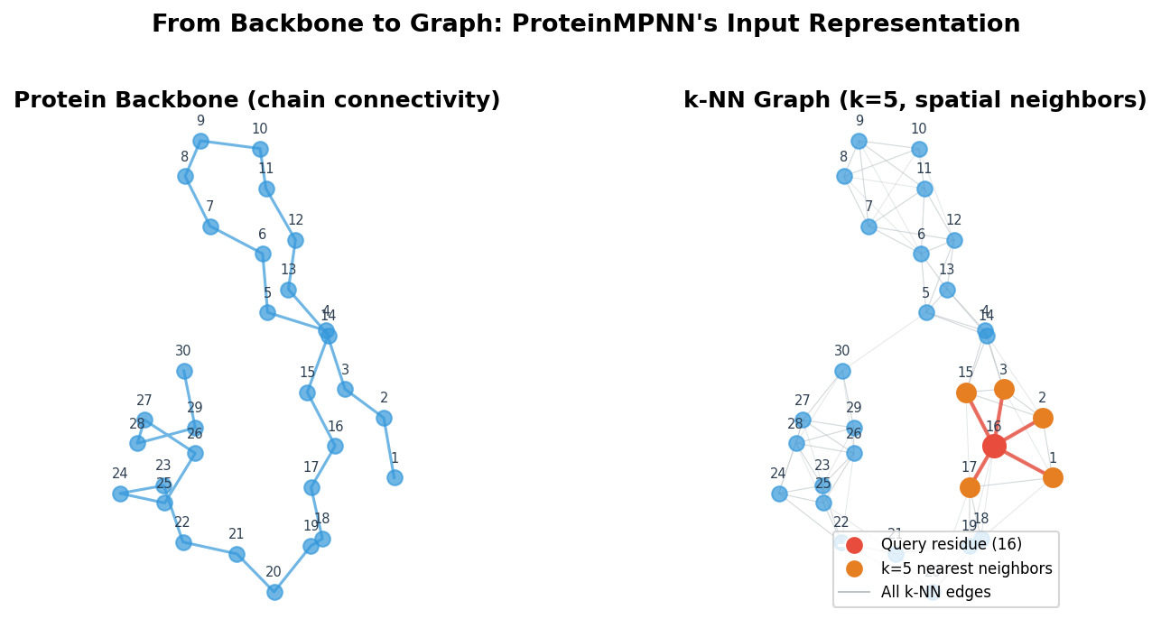
This construction captures something important about tertiary structure. Two residues that are 50 positions apart in the sequence might be less than 5 angstroms apart in space because the chain has folded back on itself. By using spatial rather than sequence neighborhoods, the graph encodes exactly these long-range contacts that define the protein’s three-dimensional shape.
3. Edge Features: Encoding Spatial Relationships
A single distance number between two residues is not enough to describe their geometric relationship. Two residue pairs might both be 8 angstroms apart, yet one pair could be in a parallel beta-sheet (side by side, pointing the same direction) while the other is in an antiparallel arrangement (side by side, pointing opposite directions). ProteinMPNN uses a rich set of edge features to capture these distinctions.
Radial Basis Function (RBF) Distance Encoding
Rather than feeding the raw distance to the network, ProteinMPNN passes it through a set of Gaussian basis functions. Given a distance \(d\), the RBF encoding produces a vector:
\[\text{RBF}(d) = \left[\exp\left(-\gamma (d - \mu_1)^2\right),\; \exp\left(-\gamma (d - \mu_2)^2\right),\; \dots,\; \exp\left(-\gamma (d - \mu_K)^2\right)\right]\]where \(\mu_1, \mu_2, \dots, \mu_K\) are evenly spaced centers between 0 and a maximum distance (e.g., 20 angstroms), and \(\gamma\) controls the width of each Gaussian. This encoding is smooth and differentiable, and it allows the network to treat different distance ranges with separate learned weights.
def rbf_encode(distances, num_rbf=16, max_dist=20.0):
    """
    Encode distances using radial basis functions.

    Args:
        distances: [E] tensor of pairwise distances.
        num_rbf: Number of Gaussian basis functions.
        max_dist: Maximum distance covered by the basis centers.

    Returns:
        rbf: [E, num_rbf] tensor of RBF-encoded distances.
    """
    centers = torch.linspace(0, max_dist, num_rbf, device=distances.device)
    gamma = num_rbf / max_dist
    return torch.exp(-gamma * (distances.unsqueeze(-1) - centers) ** 2)
Local Coordinate Frames
Each residue has a natural local coordinate system defined by its three backbone atoms: N, \(\text{C}_\alpha\), and C. These three atoms define a plane, and from that plane we can construct an orthonormal frame3:
- The x-axis points from \(\text{C}_\alpha\) toward C.
- The z-axis is perpendicular to the N-\(\text{C}_\alpha\)-C plane (computed via a cross product).
- The y-axis completes the right-handed coordinate system.
def compute_local_frame(N, CA, C):
    """
    Compute a local coordinate frame from backbone atoms N, CA, C.

    Args:
        N:  [..., 3] nitrogen positions.
        CA: [..., 3] alpha-carbon positions.
        C:  [..., 3] carbonyl carbon positions.

    Returns:
        R: [..., 3, 3] rotation matrix (columns are x, y, z axes).
        t: [..., 3] translation (the CA position).
    """
    # x-axis: CA -> C direction
    x = C - CA
    x = x / (x.norm(dim=-1, keepdim=True) + 1e-8)

    # z-axis: perpendicular to the N-CA-C plane
    v = N - CA
    z = torch.cross(x, v, dim=-1)
    z = z / (z.norm(dim=-1, keepdim=True) + 1e-8)

    # y-axis: completes the right-handed frame
    y = torch.cross(z, x, dim=-1)

    R = torch.stack([x, y, z], dim=-1)  # [..., 3, 3]
    return R, CA
Direction and Orientation Features
Using the local frames, ProteinMPNN computes several additional edge features for each pair of connected residues \(i\) and \(j\):
- Direction vectors. The vector from residue \(i\) to residue \(j\), expressed in residue \(i\)’s local frame (and vice versa). This tells the network whether neighbor \(j\) is “in front of,” “behind,” “above,” or “below” residue \(i\).
- Orientation features. Dot products between the axes of frames \(i\) and \(j\). These capture whether two residues are pointing in the same direction, perpendicular to each other, or antiparallel.
- Sequence separation. The difference \(\lvert j - i \rvert\) in sequence position. This distinguishes local contacts (expected from chain connectivity) from long-range contacts (which carry more structural information).
Together, these features give the network a rich geometric vocabulary. Rather than learning from scratch what an “alpha helix” or “beta sheet” looks like, the network receives information that already encodes many of the relevant structural motifs.
4. The Structure Encoder: Message Passing
With the graph constructed and edge features computed, the structure encoder integrates information across the protein. Its mechanism is message passing—a paradigm from graph neural networks where each node iteratively gathers information from its neighbors4.
How Message Passing Works
Each node (residue) in the graph maintains a feature vector \(\mathbf{h}_i\). At each layer of the encoder, three operations occur:
-
Message computation. For each edge \((i, j)\), a message \(\mathbf{m}_{j \to i}\) is computed from the features of both endpoints and the edge:
\[\mathbf{m}_{j \to i} = f_{\text{msg}}\!\left(\mathbf{h}_i,\; \mathbf{h}_j,\; \mathbf{e}_{ij}\right)\]where \(f_{\text{msg}}\) is a learned MLP and \(\mathbf{e}_{ij}\) is the edge feature vector.
-
Aggregation. Each residue sums the messages from all its neighbors:
\[\mathbf{a}_i = \sum_{j \in \mathcal{N}(i)} \mathbf{m}_{j \to i}\]The sum is permutation-invariant—the order of neighbors does not matter.
-
Update. Each residue updates its feature vector using its old state and the aggregated messages:
\[\mathbf{h}_i^{(\ell+1)} = f_{\text{upd}}\!\left(\mathbf{h}_i^{(\ell)},\; \mathbf{a}_i\right)\]with residual connections and layer normalization for stable training.
After \(\ell\) layers, each residue’s representation encodes information from residues up to \(\ell\) hops away in the graph. With \(k = 30\) neighbors and 3 layers (the typical depth in ProteinMPNN), the receptive field covers a substantial portion of the protein’s local structural environment.
class MPNNLayer(nn.Module):
    """Single message-passing layer for the structure encoder."""

    def __init__(self, hidden_dim, dropout=0.1):
        super().__init__()
        self.hidden_dim = hidden_dim

        # Message function: takes [h_i, h_j, e_ij] and produces a message vector
        self.message_mlp = nn.Sequential(
            nn.Linear(hidden_dim * 3, hidden_dim),
            nn.ReLU(),
            nn.Linear(hidden_dim, hidden_dim),
            nn.Dropout(dropout),
        )

        # Update function: takes [h_i, aggregated_messages] and produces updated h_i
        self.update_mlp = nn.Sequential(
            nn.Linear(hidden_dim * 2, hidden_dim),
            nn.ReLU(),
            nn.Linear(hidden_dim, hidden_dim),
            nn.Dropout(dropout),
        )

        self.norm1 = nn.LayerNorm(hidden_dim)
        self.norm2 = nn.LayerNorm(hidden_dim)

    def forward(self, h, e, edge_index):
        """
        Args:
            h: [L, hidden_dim] node features for L residues.
            e: [E, hidden_dim] edge features for E edges.
            edge_index: [2, E] source and destination indices.

        Returns:
            h_new: [L, hidden_dim] updated node features.
        """
        src, dst = edge_index
        L = h.shape[0]

        # Step 1: Compute messages m_{src -> dst}
        msg_input = torch.cat([h[src], h[dst], e], dim=-1)
        messages = self.message_mlp(msg_input)  # [E, hidden_dim]

        # Step 2: Aggregate messages at each destination node
        aggregated = torch.zeros(L, self.hidden_dim, device=h.device)
        aggregated.scatter_add_(
            0, dst.unsqueeze(-1).expand(-1, self.hidden_dim), messages
        )

        # Step 3: Update node features with residual connection
        h_res = self.norm1(h + aggregated)
        h_new = h_res + self.update_mlp(torch.cat([h_res, aggregated], dim=-1))
        h_new = self.norm2(h_new)

        return h_new
After three such layers, each residue’s representation captures not just its own local geometry but the shape of nearby secondary structure elements, the positioning of core versus surface, and the presence of cavities or channels. This contextual encoding is the foundation on which the decoder builds.
flowchart TB
    subgraph Encoder["3-Layer Message Passing Encoder"]
        direction LR
        L1["Layer 1\n(local geometry)"] --> L2["Layer 2\n(secondary structure\ncontext)"] --> L3["Layer 3\n(tertiary structure\ncontext)"]
    end

    IN["Node features\n(backbone angles,\npositions)"] --> Encoder
    EDGE["Edge features\n(distances,\norientations)"] --> Encoder
    Encoder --> OUT["Context-aware\nresidue embeddings\n(L × d)"]

    style Encoder fill:#fff3e0,stroke:#FF9800
5. Autoregressive Decoding: One Amino Acid at a Time
flowchart LR
    subgraph Decode["Autoregressive Decoding"]
        direction LR
        S1["Position 1:\nP(s₁|X)"] --> S2["Position 2:\nP(s₂|s₁, X)"]
        S2 --> S3["Position 3:\nP(s₃|s₁,s₂, X)"]
        S3 --> DOTS["..."]
        DOTS --> SL["Position L:\nP(s_L|s₁...s_{L-1}, X)"]
    end

    ENC["Encoder\nembeddings"] --> Decode
    Decode --> SEQ["Designed\nSequence"]

    style S1 fill:#e8f5e9,stroke:#4CAF50
    style S2 fill:#e8f5e9,stroke:#4CAF50
    style S3 fill:#e8f5e9,stroke:#4CAF50
    style SL fill:#e8f5e9,stroke:#4CAF50
Given the encoded structure, ProteinMPNN generates a sequence autoregressively: one amino acid at a time, where each prediction depends on all previous predictions.
The Autoregressive Factorization
Let \(\mathbf{s} = (s_1, s_2, \dots, s_L)\) denote the sequence and \(\mathcal{X}\) the backbone structure. The autoregressive approach factorizes the joint probability as:
\[P(\mathbf{s} \mid \mathcal{X}) = \prod_{i=1}^{L} P\!\left(s_{\pi(i)} \mid s_{\pi(1)}, \dots, s_{\pi(i-1)},\; \mathcal{X}\right)\]where \(\pi\) is a permutation that defines the decoding order (discussed below). Each factor represents the probability of the amino acid at position \(\pi(i)\), conditioned on the backbone structure and all amino acids decoded before it.
This factorization has three advantages over predicting all positions simultaneously5:
- Captures dependencies. If you place a positively charged lysine at one position, a nearby position might prefer a negatively charged glutamate for favorable electrostatic interaction. Autoregressive generation models these pairwise preferences naturally.
- Exact likelihoods. We can compute \(\log P(\mathbf{s} \mid \mathcal{X})\) exactly by summing the log-probabilities at each step. This is useful for ranking and filtering designs.
- Flexible constraints. We can fix certain positions, adjust sampling randomness, or apply other constraints during generation without retraining.
Random Decoding Order
In language models, we generate tokens left to right because that matches how we read. For proteins, there is no privileged direction—the N-terminus is not inherently more important than the C-terminus.
ProteinMPNN uses a random decoding order during training. Each training example uses a different random permutation \(\pi\). This has three important consequences:
- Order-agnostic learning. The model learns to predict any position given any subset of other positions, making it flexible at inference time.
- Bidirectional context. When decoding position \(i\), the model may have already decoded positions both before and after \(i\) in the sequence. This provides richer context than strict left-to-right generation.
- Reduced bias. N-to-C decoding would create an asymmetry where early positions are predicted with less context than late positions. Random order averages out this bias over many training iterations.
The decoding order is enforced through a causal mask that prevents each position from attending to positions that have not yet been decoded:
def create_decoding_mask(decoding_order):
    """
    Create a causal attention mask for an arbitrary decoding order.

    Args:
        decoding_order: [L] tensor. decoding_order[step] = position decoded at that step.

    Returns:
        mask: [L, L] boolean tensor.
              mask[i, j] = True means position i CANNOT attend to position j.
    """
    L = decoding_order.shape[0]

    # order_idx[pos] = the step at which position pos is decoded
    order_idx = torch.zeros(L, dtype=torch.long, device=decoding_order.device)
    order_idx[decoding_order] = torch.arange(L, device=decoding_order.device)

    # Position i can attend to position j only if j was decoded before i
    # i.e., order_idx[j] < order_idx[i]
    mask = order_idx.unsqueeze(0) >= order_idx.unsqueeze(1)  # [L, L]

    return mask
Sampling Strategies
Once the model is trained, we control the diversity of generated sequences through sampling strategies that adjust the trade-off between confidence and exploration.
Temperature sampling. Let \(z_i\) denote the logit (raw network output) for amino acid \(i\). The sampling probability is:
\[P(s = i) = \frac{\exp(z_i / T)}{\sum_{j=1}^{20} \exp(z_j / T)}\]where \(T\) is the temperature. When \(T < 1\), the distribution sharpens toward the most likely amino acid. When \(T > 1\), the distribution flattens, giving rare amino acids a higher chance. In practice, temperatures of 0.1–0.3 produce conservative, high-confidence designs; temperatures near 1.0 explore more diverse alternatives.
Top-\(k\) sampling. Only consider the \(k\) amino acids with the highest logits; set all other probabilities to zero. This prevents sampling extremely unlikely amino acids while preserving diversity among the top choices.
Top-\(p\) (nucleus) sampling. Select the smallest set of amino acids whose cumulative probability exceeds a threshold \(p\). If one amino acid dominates (e.g., 95% probability), only that amino acid is considered. If the distribution is flat, many amino acids remain in the candidate set. This adaptive behavior makes top-\(p\) sampling more robust than a fixed top-\(k\).
def sample_sequence(model, structure_encoding, temperature=0.1,
                    top_k=None, decoding_order=None):
    """
    Sample a complete amino acid sequence from ProteinMPNN.

    Args:
        model: Trained ProteinMPNN model.
        structure_encoding: [L, hidden_dim] encoded backbone features.
        temperature: Sampling temperature (lower = more deterministic).
        top_k: If set, only consider the top-k most likely amino acids.
        decoding_order: [L] permutation. Random if None.

    Returns:
        sequence:  [L] tensor of sampled amino acid indices (0-19).
        log_probs: [L] tensor of log-probabilities at each position.
    """
    L = structure_encoding.shape[0]
    device = structure_encoding.device
    NUM_AMINO_ACIDS = 20
    MASK_TOKEN = 21  # special token for "not yet decoded"

    if decoding_order is None:
        decoding_order = torch.randperm(L, device=device)

    sequence = torch.full((L,), MASK_TOKEN, device=device, dtype=torch.long)
    log_probs = torch.zeros(L, device=device)

    for step in range(L):
        pos = decoding_order[step].item()

        # Get logits for this position, conditioned on structure + decoded residues
        mask = create_decoding_mask(decoding_order[:step + 1])
        logits = model.decoder(
            structure_encoding.unsqueeze(0),
            sequence.unsqueeze(0),
            decoding_order,
            mask,
        )
        logits = logits[0, pos, :NUM_AMINO_ACIDS]  # [20]

        # Apply temperature
        logits = logits / temperature

        # Optional top-k filtering
        if top_k is not None:
            topk_vals, topk_idx = logits.topk(top_k)
            logits = torch.full_like(logits, float('-inf'))
            logits[topk_idx] = topk_vals

        # Sample from the distribution
        probs = torch.softmax(logits, dim=-1)
        aa = torch.multinomial(probs, num_samples=1).item()

        sequence[pos] = aa
        log_probs[pos] = torch.log(probs[aa])

    return sequence, log_probs
6. Training: Learning from Nature’s Designs
Training ProteinMPNN is conceptually straightforward: show the model millions of protein structures paired with their natural sequences, and train it to predict the sequence given the structure. Several details make this work well in practice.
Loss Function
The training objective is the negative log-likelihood of the true sequence under the model’s autoregressive distribution:
\[\mathcal{L} = -\sum_{i=1}^{L} \log P\!\left(s_i^{\text{true}} \mid s_{<i}^{\text{true}},\; \mathcal{X}\right)\]This is equivalent to cross-entropy loss between the predicted amino acid probabilities and the true amino acids at each position. During training, the model uses teacher forcing: it conditions on the true previous amino acids rather than its own predictions, which makes training efficient and fully parallelizable across positions.
Random Order Training
At each training iteration, a fresh random permutation \(\pi\) is sampled for each protein in the batch. This ensures the model cannot rely on a fixed decoding direction and must learn to predict any position given any subset of context positions.
def train_step(model, batch, optimizer, device):
    """
    One training step for ProteinMPNN.

    Args:
        model: The ProteinMPNN model.
        batch: Dictionary with 'coords' (backbone atoms) and 'sequence' (true AAs).
        optimizer: PyTorch optimizer.
        device: Computation device.

    Returns:
        loss: Scalar training loss for this batch.
    """
    model.train()

    coords = {k: v.to(device) for k, v in batch['coords'].items()}
    sequence = batch['sequence'].to(device)  # [L] true amino acid indices
    L = sequence.shape[0]

    # Sample a fresh random decoding order for this example
    decoding_order = torch.randperm(L, device=device)

    # Forward pass: predict amino acid logits at each position
    logits = model(coords, sequence, decoding_order)  # [L, 20]

    # Cross-entropy loss against the true sequence
    loss = nn.functional.cross_entropy(
        logits.view(-1, 20),
        sequence.view(-1),
        reduction='mean',
    )

    optimizer.zero_grad()
    loss.backward()
    optimizer.step()

    return loss.item()
Data Augmentation
Real experimental structures contain measurement errors, conformational flexibility, and occasional mistakes. ProteinMPNN uses two forms of data augmentation to build robustness:
Coordinate noise. Small Gaussian noise (standard deviation \(\sim\) 0.1 angstroms) is added to backbone atom positions. This simulates the uncertainty in experimental coordinates and prevents the model from relying on overly precise geometric details that would not be present in computationally designed backbones.
Random cropping. Training on random contiguous segments of proteins helps the model generalize across protein sizes and prevents memorization of specific proteins.
def augment_structure(coords, noise_prob=0.1, noise_std=0.1):
    """
    Add Gaussian noise to backbone coordinates with some probability.

    Args:
        coords: Dictionary mapping atom names ('N', 'CA', 'C', 'O') to [L, 3] tensors.
        noise_prob: Probability of applying noise.
        noise_std: Standard deviation of Gaussian noise in angstroms.

    Returns:
        coords: Augmented coordinates (modified in-place).
    """
    if torch.rand(1).item() < noise_prob:
        for atom_name in coords:
            coords[atom_name] = coords[atom_name] + torch.randn_like(coords[atom_name]) * noise_std
    return coords
Training Data
The original ProteinMPNN was trained on experimentally determined protein structures from the Protein Data Bank (PDB). The training set includes tens of thousands of protein chains spanning diverse folds, sizes, and functions. Structures are filtered by resolution (typically \(\leq\) 3.5 angstroms) and redundancy (removing near-identical chains) to ensure a high-quality, non-redundant training set.
7. Advanced Features: Constraints and Symmetry
Real protein design problems come with constraints. You may need to keep certain catalytic residues unchanged, or you may be designing a symmetric oligomer where all chains must share the same sequence. ProteinMPNN handles both cases cleanly.
Fixed Position Conditioning
Suppose you have a validated binding interface and want to redesign only the rest of the protein for improved stability. The approach is simple: set the binding-site residues to their known amino acids and exclude them from the decoding order. The decoder then conditions on these fixed positions when generating the remaining sequence.
def design_with_fixed_positions(model, coords, fixed_positions, fixed_aas):
    """
    Design a sequence with certain positions held fixed.

    Args:
        model: Trained ProteinMPNN.
        coords: Dictionary of backbone coordinates.
        fixed_positions: List of residue indices to keep fixed.
        fixed_aas: List of amino acid indices at those positions.

    Returns:
        sequence: [L] tensor of amino acid indices.
    """
    L = coords['CA'].shape[0]
    structure_encoding = model.encode(coords)

    MASK_TOKEN = 21
    sequence = torch.full((L,), MASK_TOKEN, dtype=torch.long)

    # Pre-fill fixed positions
    for pos, aa in zip(fixed_positions, fixed_aas):
        sequence[pos] = aa

    # Decoding order: fixed positions first (already known), then free positions
    free_positions = [i for i in range(L) if i not in fixed_positions]
    decoding_order = torch.tensor(
        list(fixed_positions) + free_positions, dtype=torch.long
    )

    # Decode only the free positions
    for step in range(len(fixed_positions), L):
        pos = decoding_order[step].item()

        mask = create_decoding_mask(decoding_order[:step + 1])
        logits = model.decoder(
            structure_encoding.unsqueeze(0),
            sequence.unsqueeze(0),
            decoding_order,
            mask,
        )

        aa = logits[0, pos].argmax().item()
        sequence[pos] = aa

    return sequence
This mechanism is powerful because it lets you mix experimental knowledge (known functional residues) with computational design (optimized scaffold residues) in a single pass.
Tied Positions for Symmetric Assemblies
Symmetric protein assemblies—homodimers, homotrimers, and larger oligomers—consist of multiple copies of the same chain. All copies must have identical sequences, but they occupy different spatial positions in the complex. ProteinMPNN handles this through tied positions6.
The strategy is to group positions that must share the same amino acid (corresponding positions across symmetric copies), then decode only one representative from each group. At each decoding step, the chosen amino acid is copied to all tied partners:
def design_with_symmetry(model, coords, symmetry_groups):
    """
    Design a sequence with symmetry constraints.

    Args:
        model: Trained ProteinMPNN.
        coords: Backbone coordinates for the full assembly.
        symmetry_groups: List of lists. Each inner list contains positions
                         that must have the same amino acid.

    Returns:
        sequence: [L] tensor of amino acid indices.
    """
    L = coords['CA'].shape[0]
    structure_encoding = model.encode(coords)

    MASK_TOKEN = 21
    sequence = torch.full((L,), MASK_TOKEN, dtype=torch.long)

    # Decode only the first representative from each symmetry group
    representatives = [group[0] for group in symmetry_groups]
    decoding_order = torch.tensor(representatives, dtype=torch.long)

    for step, pos in enumerate(representatives):
        mask = create_decoding_mask(decoding_order[:step + 1])
        logits = model.decoder(
            structure_encoding.unsqueeze(0),
            sequence.unsqueeze(0),
            decoding_order,
            mask,
        )

        aa = logits[0, pos].argmax().item()

        # Copy the chosen amino acid to all symmetric partners
        for group in symmetry_groups:
            if pos in group:
                for tied_pos in group:
                    sequence[tied_pos] = aa
                break

    return sequence
This approach is efficient—the number of decoding steps equals the number of unique positions, not the total number of residues—and it guarantees that all symmetry-related positions receive the same amino acid.
8. The Design Pipeline: RFDiffusion + ProteinMPNN + AlphaFold
flowchart LR
    SPEC["Design\nSpecification"] --> RFD["RFDiffusion\n(backbone\ngeneration)"]
    RFD --> BB["Backbone\nStructures"]
    BB --> MPNN["ProteinMPNN\n(inverse folding)"]
    MPNN --> SEQS["Candidate\nSequences"]
    SEQS --> AF["AlphaFold2\n(structure\nprediction)"]
    AF --> VAL{"TM-score\n> 0.8?"}
    VAL -->|"Yes"| EXP["Experimental\nValidation\n(express & test)"]
    VAL -->|"No"| FILTER["Discard"]

    style RFD fill:#fce4ec,stroke:#e91e63
    style MPNN fill:#e8f5e9,stroke:#4CAF50
    style AF fill:#e8f4fd,stroke:#2196F3
    style EXP fill:#fff3e0,stroke:#FF9800
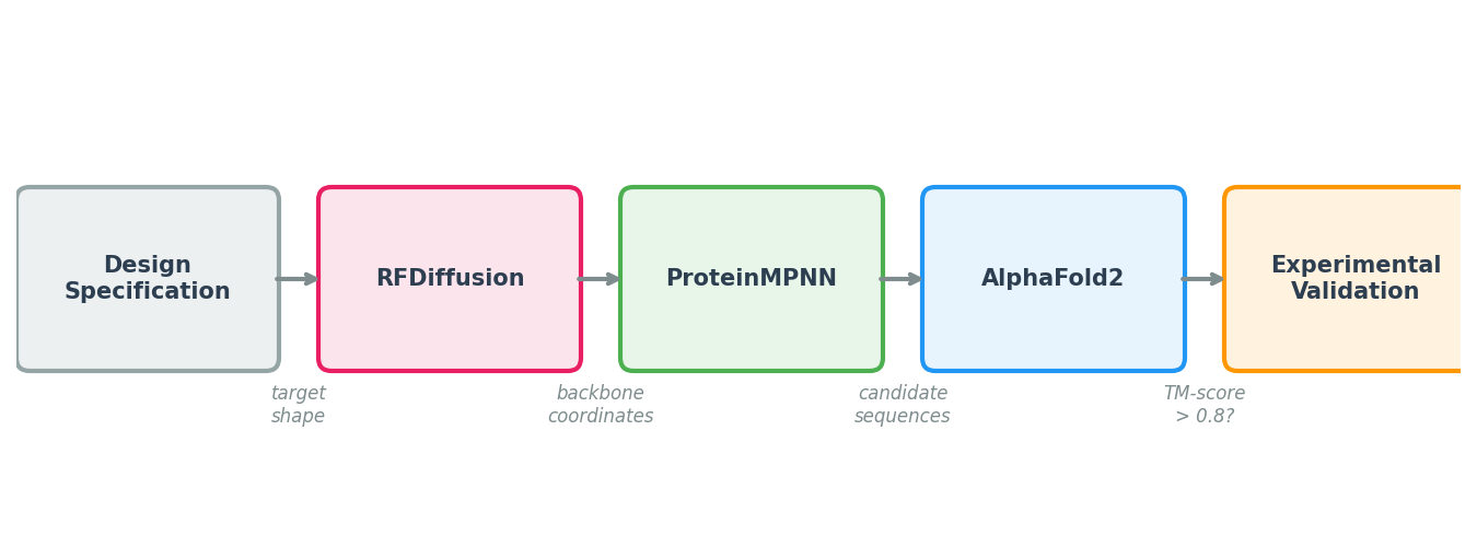
ProteinMPNN’s impact comes from its role in a larger pipeline. No single tool handles the full journey from design specification to experimentally validated protein. The modern computational protein design workflow chains three models together, each solving a different sub-problem.
Step 1: Backbone Generation with RFDiffusion
The pipeline begins with a design specification: a binder to a specific epitope, a symmetric assembly, or an enzyme scaffold with catalytic residues at defined positions. RFDiffusion (Lecture 5) takes this specification and generates diverse backbone structures—sets of \((\text{N}, \text{C}_\alpha, \text{C}, \text{O})\) coordinates for each residue—that satisfy the specification.
At this stage, the output is purely geometric. There are no amino acid identities, only a shape.
Step 2: Sequence Design with ProteinMPNN
For each backbone from Step 1, ProteinMPNN generates multiple candidate sequences. Practical recommendations:
- Generate many candidates. ProteinMPNN is fast. Generate 100 or more sequences per backbone, then filter aggressively. The computational cost is negligible compared to the cost of a failed experiment.
- Use multiple temperatures. Generate some sequences at low temperature (\(T = 0.1\), conservative, high confidence) and some at higher temperature (\(T = 0.3\text{--}1.0\), diverse, potentially discovering better solutions). The optimal temperature depends on the application.
- Apply constraints. If certain residues are functionally required (e.g., catalytic triads, disulfide bonds), fix them during decoding.
Step 3: Validation with AlphaFold or ESMFold
The key question is: will the designed sequence actually fold into the intended backbone? To answer this, we run the designed sequence through a structure prediction model—AlphaFold2 (Lecture 4) or ESMFold—and compare the predicted structure to the design target.
The primary metric is the TM-score7, which measures global structural similarity on a scale from 0 (unrelated) to 1 (identical). A TM-score above 0.5 generally indicates that two structures share the same fold; designs with TM-scores above 0.8 are considered high-confidence matches. AlphaFold’s per-residue confidence score (pLDDT) provides additional information about which regions of the design are well-predicted.
Step 4: Filtering and Ranking
After structure prediction, filter and rank candidates using:
- TM-score between the predicted and designed backbones.
- pLDDT from AlphaFold (higher is better; values above 80 suggest confident predictions).
- Sequence properties such as predicted solubility, aggregation propensity, and expression likelihood.
- Diversity among the top candidates, to maximize the chance that at least one works experimentally.
Step 5: Experimental Validation
The final step is synthesis and testing. Selected sequences are ordered as synthetic genes, cloned into expression vectors, expressed in cells (typically E. coli or mammalian cell lines), purified, and tested for the intended function.
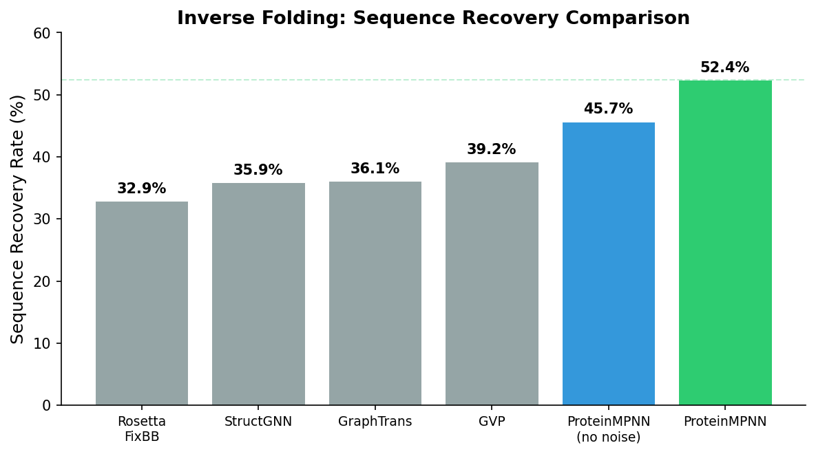
The original ProteinMPNN paper reported that over 50% of designed sequences folded into the target structure when tested experimentally—a dramatic improvement over previous methods, which achieved roughly 10% success rates. This high hit rate makes the RFDiffusion \(\to\) ProteinMPNN \(\to\) AlphaFold pipeline practical for real-world protein engineering.
Pipeline Summary
Step 1: RFDiffusion
   Specification  -->  Backbone coordinates

Step 2: ProteinMPNN
   Backbone  -->  100+ candidate sequences (diverse temperatures)

Step 3: AlphaFold / ESMFold
   Each sequence  -->  Predicted structure + confidence (pLDDT)

Step 4: Filtering
   Keep sequences where predicted structure matches design (TM-score > 0.8)

Step 5: Experiment
   Synthesize, express, purify, test
Practical Considerations
Consider the full biological context. ProteinMPNN designs sequences for isolated chains or complexes, but the protein will eventually exist inside a cell or in a buffer. Check for protease cleavage sites, glycosylation motifs, and compatibility with your expression system.
Iterate. The pipeline is fast enough to run multiple rounds. If early designs fail, analyze the failures, adjust constraints, and redesign. Each round provides information that improves subsequent attempts.
9. Design Principles and Alternatives
What Makes ProteinMPNN Work
Several design choices contribute to ProteinMPNN’s effectiveness. The table below summarizes them:
| Principle | Implementation | Why It Works |
|---|---|---|
| Structure as graph | k-NN graph on \(\text{C}_\alpha\) atoms | Captures both local and long-range spatial contacts |
| Rich edge features | RBF distances, local frames, orientations | Provides geometric vocabulary beyond raw distances |
| Autoregressive decoding | One amino acid per step | Models inter-residue dependencies accurately |
| Random decoding order | Fresh permutation each training step | Prevents directional bias; enables flexible generation |
| Controlled sampling | Temperature, top-\(k\), top-\(p\) | Balances sequence diversity against design confidence |
Feature Engineering Still Matters
ProteinMPNN’s success relies on carefully designed geometric features—local coordinate frames, RBF-encoded distances, orientation dot products. These features provide the network with a structural vocabulary that would take far more data and capacity to learn from raw coordinates alone. This is an instructive counterpoint to the “end-to-end learning” philosophy: in domains with strong geometric structure, thoughtful feature engineering remains a powerful tool.
Comparison with Alternative Methods
ProteinMPNN is not the only inverse folding method. Understanding the alternatives clarifies its design choices:
| Method | Approach | Key Strength |
|---|---|---|
| ProteinMPNN (Dauparas et al., 2022) | Autoregressive GNN | High accuracy, fast inference, widely adopted |
| ESM-IF (Hsu et al., 2022) | Transformer + ESM language model backbone | Leverages evolutionary knowledge from large-scale pre-training |
| GVP (Jing et al., 2021) | Geometric vector perceptrons | Built-in SE(3) equivariance without data augmentation |
| AlphaDesign | AlphaFold-based end-to-end | Differentiable structure-aware loss |
ProteinMPNN’s combination of accuracy, speed, and simplicity has made it the de facto standard. It runs in seconds per sequence on a single GPU, requires no MSA computation, and integrates seamlessly into the RFDiffusion pipeline.
10. Exercises
The following exercises range from conceptual questions to implementation tasks. They are designed to solidify your understanding of the concepts covered in this lecture.
Conceptual Questions
Exercise 1: Many-to-One Mapping. Hemoglobin proteins across species share the same fold despite less than 50% sequence identity. Explain, in terms of the types of amino acid positions in a protein (core, surface, functional), why such large sequence variation is tolerated. How does ProteinMPNN exploit this redundancy?
Exercise 2: Decoding Order. Suppose ProteinMPNN were trained with a fixed N-to-C decoding order instead of random order. Describe two specific failure modes you would expect at inference time. Would the model be more or less suitable for fixed-position conditioning? Explain your reasoning.
Exercise 3: Temperature Trade-offs. You are designing a therapeutic protein binder using the RFDiffusion \(\to\) ProteinMPNN \(\to\) AlphaFold pipeline. You have budget for 10 experimental candidates. Would you generate all 10 at low temperature (\(T = 0.1\)), all 10 at high temperature (\(T = 1.0\)), or a mix? Justify your strategy.
Implementation Tasks
Exercise 4: Tied Sampling with Logit Averaging. Extend the design_with_symmetry function so that, instead of using logits from only the representative position, it averages the logits across all positions in the symmetry group before sampling. This should produce amino acid choices that are optimal for the structural context of all symmetric copies, not just the representative.
Hint: At each decoding step, run the decoder to get logits at all positions in the current symmetry group, then take their mean before applying softmax and sampling.
Exercise 5: Sequence Recovery Evaluation. Write a function that takes a protein structure and its known native sequence, runs ProteinMPNN (or a simplified version) to generate a sequence, and computes the sequence recovery rate—the fraction of positions where the designed amino acid matches the native amino acid. Run this for 10 proteins and report the mean and standard deviation of recovery rates.
Exercise 6: Pipeline Integration. Implement an end-to-end function that:
- Takes backbone coordinates as input.
- Generates 50 sequences with ProteinMPNN at \(T = 0.1\) and 50 sequences at \(T = 0.5\).
- Computes the mean log-probability for each sequence.
- Returns the top 10 sequences ranked by log-probability, along with their temperatures of origin.
Does low-temperature sampling always produce higher log-probability sequences? Discuss.
Exercise 7: Secondary Structure Bias. Modify the sampling function to bias certain positions toward helix-favoring amino acids (Ala, Glu, Leu, Met) or sheet-favoring amino acids (Val, Ile, Tyr, Phe) based on a provided secondary structure annotation. Implement this as an additive logit bias applied before temperature scaling.
References
-
Dauparas, J., Anishchenko, I., Bennett, N., Baek, M., et al. (2022). “Robust deep learning-based protein sequence design using ProteinMPNN.” Science, 378(6615), 49–56. doi:10.1126/science.add2187
-
Watson, J. L., Juergens, D., Bennett, N. R., Trippe, B. L., et al. (2023). “De novo design of protein structure and function with RFdiffusion.” Nature, 620, 1089–1100. doi:10.1038/s41586-023-06415-8
-
Hsu, C., Verkuil, R., Liu, J., Lin, Z., Rives, A., et al. (2022). “Learning inverse folding from millions of predicted structures.” Proceedings of the 39th International Conference on Machine Learning (ICML).
-
Ingraham, J., Garg, V., Barzilay, R., & Jaakkola, T. (2019). “Generative models for graph-based protein design.” Advances in Neural Information Processing Systems (NeurIPS), 32.
-
Jing, B., Eismann, S., Suriana, P., Townshend, R. K. L., & Dror, R. (2021). “Learning from Protein Structure with Geometric Vector Perceptrons.” International Conference on Learning Representations (ICLR).
-
Gilmer, J., Schoenholz, S. S., Riley, P. F., Vinyals, O., & Dahl, G. E. (2017). “Neural Message Passing for Quantum Chemistry.” Proceedings of the 34th International Conference on Machine Learning (ICML).
-
Jumper, J., Evans, R., Pritzel, A., et al. (2021). “Highly accurate protein structure prediction with AlphaFold.” Nature, 596, 583–589. doi:10.1038/s41586-021-03819-2
-
The name stands for Message Passing Neural Network for Proteins. “Message passing” refers to the graph neural network mechanism at the heart of the model’s structure encoder. ↩
-
In reality, proteins sample an ensemble of conformations, but most well-folded proteins have a single dominant structure that accounts for the vast majority of the ensemble. ↩
-
This is sometimes called a residue frame or backbone frame. The same idea appears in AlphaFold’s Invariant Point Attention (Lecture 4), where each residue carries a rigid-body frame \((R_i, \mathbf{t}_i)\). ↩
-
For a review of message passing neural networks, see Gilmer et al. (2017), “Neural Message Passing for Quantum Chemistry,” ICML. We also covered the basics in Preliminary Lecture 4 (Transformers and GNNs). ↩
-
Non-autoregressive approaches do exist—for example, predicting all amino acids in parallel. These are faster at inference time but generally less accurate, because they cannot model the dependencies between positions at different steps of decoding. ↩
-
Tied positions can also enforce sequence identity between non-symmetric chains when design constraints require it, though symmetric assemblies are the most common use case. ↩
-
TM-score stands for Template Modeling score. Unlike RMSD, TM-score is length-normalized and less sensitive to local structural deviations, making it a better metric for assessing overall fold similarity. ↩