Generative Models: VAEs and Diffusion for Proteins
This is Lecture 2 of the Protein & Artificial Intelligence course (Spring 2026), co-taught by Prof. Sungsoo Ahn and Prof. Homin Kim at KAIST. The course covers core machine learning techniques for protein science, from representation learning to generative design. In this lecture we shift from discriminative models—which predict properties of existing proteins—to generative models that can imagine entirely new ones.
Introduction: Dreaming Up New Proteins
Evolution has spent roughly four billion years crafting the proteins we observe today. These molecules are the result of relentless natural selection—optimized for the particular environments and challenges their host organisms faced. Yet the proteins that exist in nature represent only a vanishing sliver of what is possible. A polypeptide chain of length 100 can be assembled from 20 standard amino acids in \(20^{100} \approx 10^{130}\) distinct ways, a number that dwarfs the roughly \(10^{80}\) atoms in the observable universe.
What lies in that unexplored space? Enzymes that degrade plastic pollutants. Binders that neutralize pandemic viruses. Molecular machines that catalyze reactions no natural enzyme has ever performed. Generative models give us a systematic way to explore this vast, uncharted territory. Instead of waiting for evolution to stumble upon useful proteins through random mutation, we can train machine learning models to internalize the statistical patterns that make proteins work—and then sample novel sequences and structures from the learned distribution.
In Lecture 1 we studied transformers and graph neural networks, architectures that process protein sequences and structures. Those were discriminative tools: given a protein, predict a property. This lecture flips the direction. We ask: given a desired property or no constraint at all, can we generate a protein that satisfies it?
We will study two foundational frameworks for generative modeling—variational autoencoders (VAEs) and denoising diffusion probabilistic models (DDPMs)—and see how each has been applied to design proteins that have never existed in nature.
Roadmap
| Section | Topic | Why It Is Needed |
|---|---|---|
| 1 | The Compression Perspective | Builds intuition for latent-variable models before any math |
| 2 | From Autoencoders to VAEs | Explains why a probabilistic latent space enables generation |
| 3 | The ELBO and Its Derivation | Provides the training objective for VAEs |
| 4 | The Reparameterization Trick | Solves the practical problem of backpropagating through sampling |
| 5 | Complete Protein VAE | Assembles a working implementation |
| 6 | Diffusion Models: Controlled Destruction | Introduces the forward noising process |
| 7 | The Reverse Process and Training Objective | Shows how the network learns to denoise |
| 8 | The Denoising Loop and Architecture | Covers generation and timestep conditioning |
| 9 | Handling Discrete Protein Data | Addresses the mismatch between Gaussian noise and discrete sequences |
| 10 | VAEs vs. Diffusion | Compares strengths, weaknesses, and computational trade-offs |
| 11 | Real-World Impact | Surveys RFDiffusion, EvoDiff, and conditional generation |
| 12 | Exercises | Hands-on practice problems |
1. The Compression Perspective
Before we write any equations, let us build intuition with a thought experiment.
Suppose you have a database of 50,000 serine protease sequences. Despite their diversity—some share less than 30% sequence identity—they all fold into similar structures, catalyze the same reaction, and place a conserved catalytic triad (Ser, His, Asp) in nearly identical spatial positions. Listing every residue of every sequence is clearly redundant. There must be a more compact description that captures the essence of what makes a serine protease a serine protease.
An autoencoder is a neural network that discovers such compact descriptions automatically. It consists of two halves:
- An encoder that compresses the input \(x\) (a protein sequence) into a low-dimensional vector \(z\), called the latent code1.
- A decoder that reconstructs the protein from \(z\).
If the network can reliably reconstruct proteins from their latent codes, those codes must contain the essential information about the input. The latent dimension is deliberately chosen to be much smaller than the input dimension, forcing the network to learn an efficient internal representation.
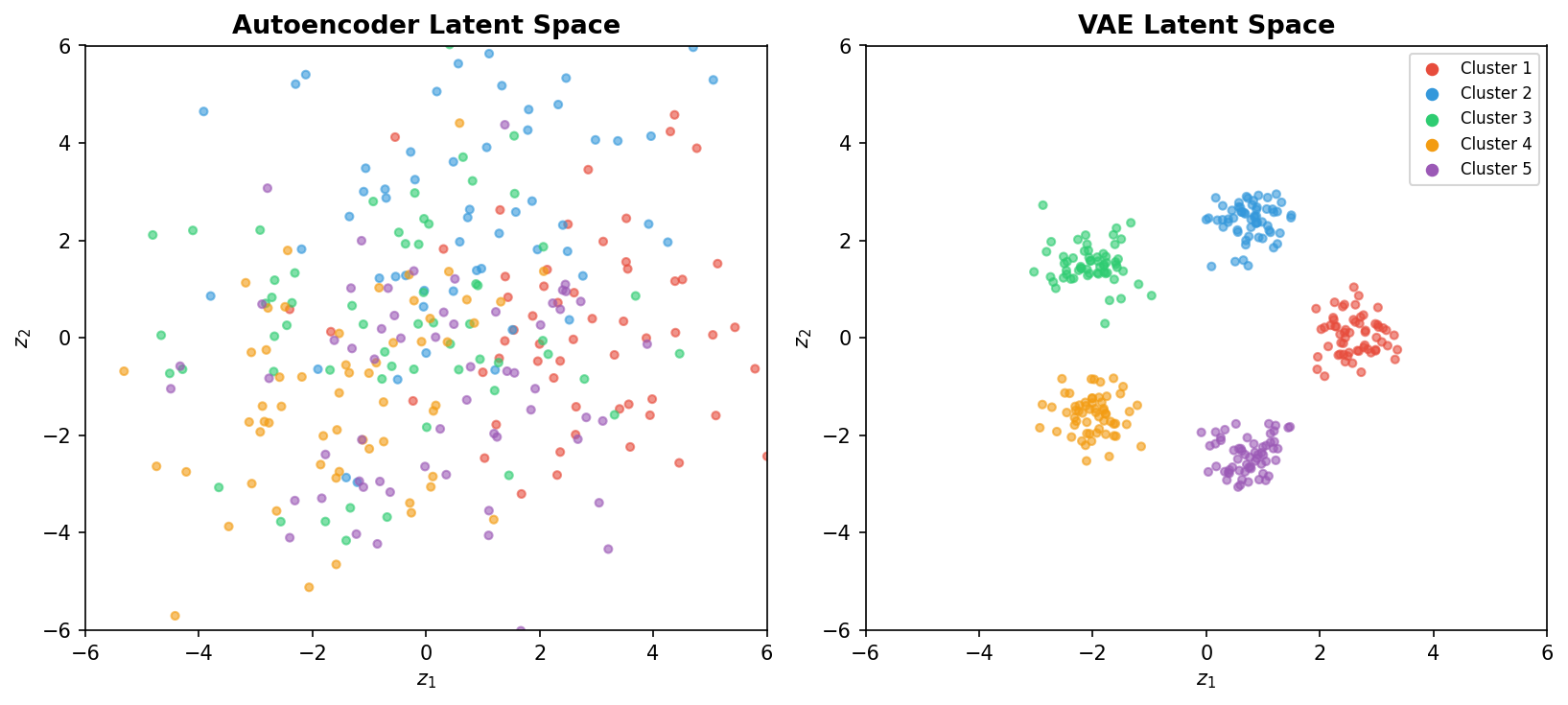
But standard autoencoders have a critical limitation for generation. Each input maps to a single, deterministic point in latent space. If we pick a random point and decode it, there is no guarantee it lies near any training example. The latent space may be riddled with gaps and dead zones—regions that decode into sequences with no physical meaning.
To see why, consider a simple analogy. Imagine plotting every serine protease as a dot in a two-dimensional space. A standard autoencoder might scatter these dots across the plane with irregular spacing. Between two clusters of dots lies empty territory. Decoding a point from that empty territory yields gibberish—a sequence that folds improperly or not at all. For generation, we need a way to make every region of latent space decode into something sensible, with smooth transitions between neighboring points.
2. From Autoencoders to VAEs
flowchart LR
    subgraph AE["Autoencoder"]
        direction LR
        X1["Input x"] --> E1["Encoder"] --> Z1["z\n(deterministic\npoint)"] --> D1["Decoder"] --> X1R["Reconstructed x̂"]
    end

    subgraph VAE["Variational Autoencoder"]
        direction LR
        X2["Input x"] --> E2["Encoder"] --> MU["μ, σ²\n(distribution\nparameters)"] --> S2["Sample\nz ~ N(μ, σ²)"] --> D2["Decoder"] --> X2R["Reconstructed x̂"]
        MU -.- KL["KL divergence\npushes toward N(0,I)"]
    end

    style Z1 fill:#fce4ec,stroke:#e91e63
    style S2 fill:#e8f5e9,stroke:#4CAF50
    style KL fill:#fff3e0,stroke:#FF9800
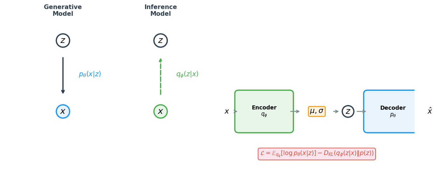
Variational autoencoders, introduced by Kingma and Welling (2014), solve this problem by making the latent space probabilistic. Instead of mapping each protein \(x\) to a single point \(z\), the encoder outputs the parameters of a Gaussian distribution—a mean vector \(\mu_\phi(x)\) and a variance vector \(\sigma^2_\phi(x)\)—from which we then sample a latent code:
\[z \sim q_\phi(z \mid x) = \mathcal{N}\!\bigl(\mu_\phi(x),\; \sigma^2_\phi(x) I\bigr)\]Here \(\phi\) denotes the learnable parameters of the encoder, \(\mathcal{N}\) is a multivariate Gaussian, and \(I\) is the identity matrix. The distribution \(q_\phi(z \mid x)\) is called the approximate posterior2 because it approximates the true (intractable) posterior \(p(z \mid x)\).
The training procedure also adds a regularizer that pushes every encoded distribution toward a standard normal \(p(z) = \mathcal{N}(0, I)\). This regularizer has a profound consequence: the entire latent space becomes populated. If we sample \(z \sim \mathcal{N}(0, I)\) and decode it, we are likely to obtain a valid protein, because the encoder has been trained to place real proteins near these regions, and the decoder has been trained to reconstruct them.
The encoder in code looks like this:
import torch
import torch.nn as nn

class ProteinEncoder(nn.Module):
    """Encodes a protein sequence into Gaussian parameters (mu, log-variance)."""

    def __init__(self, input_dim: int, hidden_dim: int, latent_dim: int):
        super().__init__()
        self.fc1 = nn.Linear(input_dim, hidden_dim)
        self.fc_mu = nn.Linear(hidden_dim, latent_dim)      # mean of q(z|x)
        self.fc_logvar = nn.Linear(hidden_dim, latent_dim)   # log-variance of q(z|x)

    def forward(self, x: torch.Tensor):
        h = torch.relu(self.fc1(x))
        mu = self.fc_mu(h)
        logvar = self.fc_logvar(h)  # outputting log(sigma^2) keeps sigma > 0
        return mu, logvar
We output \(\log \sigma^2\) rather than \(\sigma^2\) directly. Exponentiating a real number always yields a positive result, so this parameterization guarantees positive variance without needing explicit constraints.
The decoder takes a sampled latent code \(z\) and predicts a probability distribution over amino acids at each sequence position:
class ProteinDecoder(nn.Module):
    """Decodes a latent vector into amino-acid logits for each position."""

    def __init__(self, latent_dim: int, hidden_dim: int, output_dim: int):
        super().__init__()
        self.fc1 = nn.Linear(latent_dim, hidden_dim)
        self.fc2 = nn.Linear(hidden_dim, output_dim)

    def forward(self, z: torch.Tensor):
        h = torch.relu(self.fc1(z))
        return self.fc2(h)  # raw logits; softmax is applied in the loss
3. The ELBO: Deriving the Training Objective
Motivation
We want to find encoder parameters \(\phi\) and decoder parameters \(\theta\) that make our training data as probable as possible under the model. Formally, we want to maximize the marginal log-likelihood3:
\[\log p_\theta(x) = \log \int p_\theta(x \mid z)\, p(z)\, dz\]This integral sums the contributions of every possible latent code \(z\). For each \(z\), the prior \(p(z) = \mathcal{N}(0, I)\) tells us how likely that code is, and the decoder \(p_\theta(x \mid z)\) tells us how likely the protein \(x\) is given that code. Unfortunately, this integral has no closed-form solution—evaluating it would require running the decoder for every conceivable \(z\).
Deriving the Evidence Lower Bound
Variational inference sidesteps the intractable integral by deriving a tractable lower bound on \(\log p_\theta(x)\). We introduce the encoder distribution \(q_\phi(z \mid x)\) by multiplying and dividing inside the integral:
\[\log p_\theta(x) = \log \int \frac{p_\theta(x \mid z)\, p(z)}{q_\phi(z \mid x)}\; q_\phi(z \mid x)\, dz\]Recognizing the right-hand side as an expectation under \(q_\phi(z \mid x)\), we apply Jensen’s inequality4. Because \(\log\) is a concave function, we have \(\log \mathbb{E}[Y] \geq \mathbb{E}[\log Y]\) for any random variable \(Y > 0\):
\[\log p_\theta(x) \geq \int q_\phi(z \mid x) \log \frac{p_\theta(x \mid z)\, p(z)}{q_\phi(z \mid x)}\, dz\]Splitting the logarithm of the fraction yields two terms:
\[\underbrace{\int q_\phi(z \mid x) \log p_\theta(x \mid z)\, dz}_{\text{reconstruction term}} \;+\; \underbrace{\int q_\phi(z \mid x) \log \frac{p(z)}{q_\phi(z \mid x)}\, dz}_{\text{negative KL divergence}}\]Recognizing the second integral as the negative Kullback-Leibler (KL) divergence5, we arrive at the Evidence Lower Bound (ELBO):
\[\text{ELBO}(\phi, \theta; x) = \mathbb{E}_{q_\phi(z \mid x)}\!\bigl[\log p_\theta(x \mid z)\bigr] - D_{\mathrm{KL}}\!\bigl(q_\phi(z \mid x) \,\|\, p(z)\bigr)\]The relationship to the marginal log-likelihood is:
\[\log p_\theta(x) \geq \text{ELBO}\]Maximizing the ELBO pushes up on the true log-likelihood from below.
Interpreting the Two Terms
Reconstruction term \(\mathbb{E}_{q_\phi(z \mid x)}[\log p_\theta(x \mid z)]\): sample a latent code \(z\) from the encoder, pass it through the decoder, and measure how well the original protein \(x\) is recovered. Maximizing this term encourages faithful reconstruction. In practice, this is implemented as the negative cross-entropy between the decoder’s output distribution and the true amino-acid sequence.
KL term \(D_{\mathrm{KL}}(q_\phi(z \mid x) \,\|\, p(z))\): this penalizes the encoder for producing distributions that stray too far from the prior \(\mathcal{N}(0, I)\). Without this term, the encoder could assign each protein to a tiny, isolated region of latent space—perfect for reconstruction, useless for generation. The KL term forces overlapping, smooth coverage of the latent space.
Closed-Form KL for Gaussians
When both \(q_\phi(z \mid x)\) and \(p(z)\) are Gaussian, the KL divergence has a closed-form expression. Let \(q_\phi(z \mid x) = \mathcal{N}(\mu, \mathrm{diag}(\sigma^2))\) with \(\mu \in \mathbb{R}^J\) and \(\sigma \in \mathbb{R}^J\), and let \(p(z) = \mathcal{N}(0, I)\). Then:
\[D_{\mathrm{KL}} = -\frac{1}{2} \sum_{j=1}^{J} \bigl(1 + \log \sigma_j^2 - \mu_j^2 - \sigma_j^2\bigr)\]In code:
def kl_divergence(mu: torch.Tensor, logvar: torch.Tensor) -> torch.Tensor:
    """Closed-form KL divergence: KL(N(mu, sigma^2) || N(0, I)).

    Args:
        mu: encoder mean, shape [batch_size, latent_dim]
        logvar: encoder log-variance, shape [batch_size, latent_dim]

    Returns:
        KL divergence per example, shape [batch_size]
    """
    # logvar = log(sigma^2), so exp(logvar) = sigma^2
    return -0.5 * torch.sum(1 + logvar - mu.pow(2) - logvar.exp(), dim=-1)
4. The Reparameterization Trick
The Problem
Training the ELBO requires computing gradients of the reconstruction term with respect to the encoder parameters \(\phi\). But this term involves sampling \(z\) from \(q_\phi(z \mid x)\), and sampling is not a differentiable operation. Gradient-based optimizers cannot backpropagate through a random number generator.
The Solution
Kingma and Welling’s reparameterization trick rewrites the sampling step as a deterministic transformation of a fixed noise source. Instead of drawing \(z \sim \mathcal{N}(\mu, \sigma^2 I)\) directly, we draw auxiliary noise \(\epsilon \sim \mathcal{N}(0, I)\) and compute:
\[z = \mu + \sigma \odot \epsilon\]where \(\odot\) denotes element-wise multiplication. The randomness now resides entirely in \(\epsilon\), which does not depend on any learnable parameter. The mapping from \(\epsilon\) to \(z\) is a deterministic, differentiable function of \(\mu\) and \(\sigma\), so standard backpropagation applies.
Think of it this way: rather than asking “what is the gradient of a coin flip?”, we ask “what is the gradient of a shift-and-scale operation?” The latter is elementary calculus.
def reparameterize(mu: torch.Tensor, logvar: torch.Tensor) -> torch.Tensor:
    """Sample z = mu + sigma * epsilon, where epsilon ~ N(0, I).

    This makes the sampling step differentiable w.r.t. mu and logvar.
    """
    std = torch.exp(0.5 * logvar)   # sigma = exp(log(sigma^2) / 2)
    eps = torch.randn_like(std)      # epsilon ~ N(0, I)
    return mu + eps * std
5. Putting It Together: A Complete Protein VAE
We now have all the pieces. The full model takes a protein sequence (as integer-encoded amino acids), one-hot encodes it, compresses it through the encoder, samples a latent code via reparameterization, and reconstructs amino-acid logits through the decoder.
class ProteinVAE(nn.Module):
    """Variational autoencoder for fixed-length protein sequences.

    The encoder maps one-hot-encoded sequences to Gaussian parameters.
    The decoder maps sampled latent codes back to amino-acid logits.
    """

    def __init__(self, seq_len: int, vocab_size: int = 21,
                 hidden_dim: int = 256, latent_dim: int = 32):
        super().__init__()
        self.seq_len = seq_len
        self.vocab_size = vocab_size     # 20 amino acids + 1 gap/unknown
        input_dim = seq_len * vocab_size

        # Encoder: sequence -> (mu, logvar)
        self.encoder = nn.Sequential(
            nn.Linear(input_dim, hidden_dim),
            nn.ReLU(),
            nn.Linear(hidden_dim, hidden_dim),
            nn.ReLU()
        )
        self.fc_mu = nn.Linear(hidden_dim, latent_dim)
        self.fc_logvar = nn.Linear(hidden_dim, latent_dim)

        # Decoder: z -> amino-acid logits
        self.decoder = nn.Sequential(
            nn.Linear(latent_dim, hidden_dim),
            nn.ReLU(),
            nn.Linear(hidden_dim, hidden_dim),
            nn.ReLU(),
            nn.Linear(hidden_dim, input_dim)
        )

    def encode(self, x: torch.Tensor):
        """Encode integer-coded sequences to Gaussian parameters."""
        x_onehot = nn.functional.one_hot(x, self.vocab_size).float()
        x_flat = x_onehot.view(x.size(0), -1)  # [batch, seq_len * vocab_size]
        h = self.encoder(x_flat)
        return self.fc_mu(h), self.fc_logvar(h)

    def decode(self, z: torch.Tensor):
        """Decode latent codes to per-position amino-acid logits."""
        h = self.decoder(z)
        return h.view(-1, self.seq_len, self.vocab_size)

    def forward(self, x: torch.Tensor):
        mu, logvar = self.encode(x)
        z = reparameterize(mu, logvar)
        recon_logits = self.decode(z)
        return recon_logits, mu, logvar

    @torch.no_grad()
    def sample(self, n_samples: int, device: str = "cpu"):
        """Generate novel sequences by sampling z ~ N(0, I) and decoding."""
        z = torch.randn(n_samples, self.fc_mu.out_features, device=device)
        logits = self.decode(z)
        return torch.argmax(logits, dim=-1)  # greedy decode
The Loss Function
The loss is the negative ELBO, averaged over the batch. An optional scaling factor \(\beta\) on the KL term (known as \(\beta\)-VAE when \(\beta \neq 1\)) trades reconstruction fidelity for a more structured latent space.
def vae_loss(recon_logits: torch.Tensor, x: torch.Tensor,
             mu: torch.Tensor, logvar: torch.Tensor,
             beta: float = 1.0):
    """Negative ELBO = reconstruction loss + beta * KL divergence.

    Args:
        recon_logits: decoder output, shape [batch, seq_len, vocab_size]
        x: ground-truth sequences, shape [batch, seq_len]
        mu, logvar: encoder outputs
        beta: weight on the KL term (beta=1 is standard VAE)

    Returns:
        total_loss, reconstruction_loss, kl_loss (all scalar tensors)
    """
    # Cross-entropy measures how well we reconstruct each amino acid
    recon_loss = nn.functional.cross_entropy(
        recon_logits.reshape(-1, recon_logits.size(-1)),
        x.reshape(-1),
        reduction="mean"
    )

    kl_loss = kl_divergence(mu, logvar).mean()
    total_loss = recon_loss + beta * kl_loss

    return total_loss, recon_loss, kl_loss
Increasing \(\beta\) above 1 pushes the encoder distributions closer to \(\mathcal{N}(0, I)\), smoothing the latent space at the expense of reconstruction accuracy.
6. Diffusion Models: Controlled Destruction
A Different Philosophy
VAEs learn generation by compressing data into a structured latent space. Diffusion models take an entirely different approach: they learn generation by learning to undo corruption.
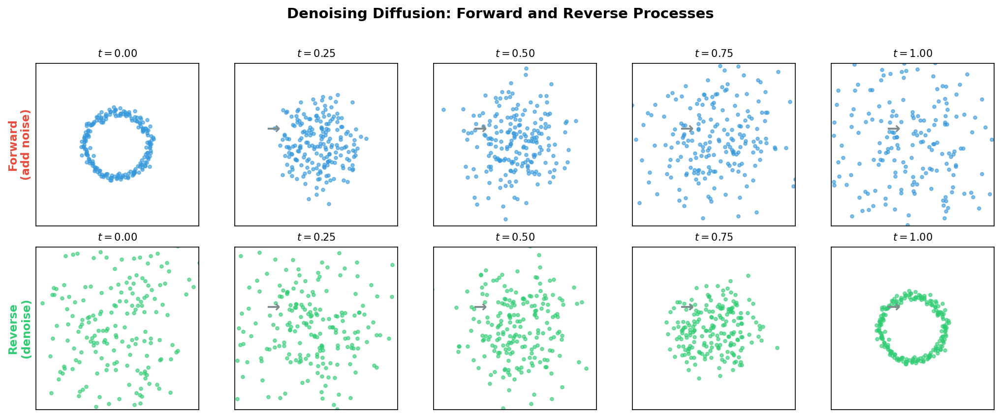
The core idea is disarmingly simple. Take a clean protein structure (or embedding), corrupt it step by step with Gaussian noise until nothing recognizable remains, and then train a neural network to reverse each corruption step.
Once trained, the network can start from pure noise and iteratively sculpt it into a realistic protein.
The intuition is that denoising is easier than generating from scratch. If someone shows you a slightly blurry photograph and asks you to sharpen it, that task is far easier than painting a photorealistic image from a blank canvas. Diffusion models decompose the hard problem of generation into many small, manageable denoising steps.
To ground this in protein science: imagine taking the 3D coordinates of a protein backbone and jittering every atom by a tiny random displacement. The resulting structure is still recognizable. A neural network that has seen many proteins could plausibly predict the original atom positions from this lightly perturbed version. Now repeat the corruption many times, adding more noise at each stage. Eventually the coordinates become indistinguishable from random points in space. But if the network can reverse each individual step—going from “slightly more noisy” to “slightly less noisy”—then chaining all the reverse steps together recovers a clean protein from pure noise.
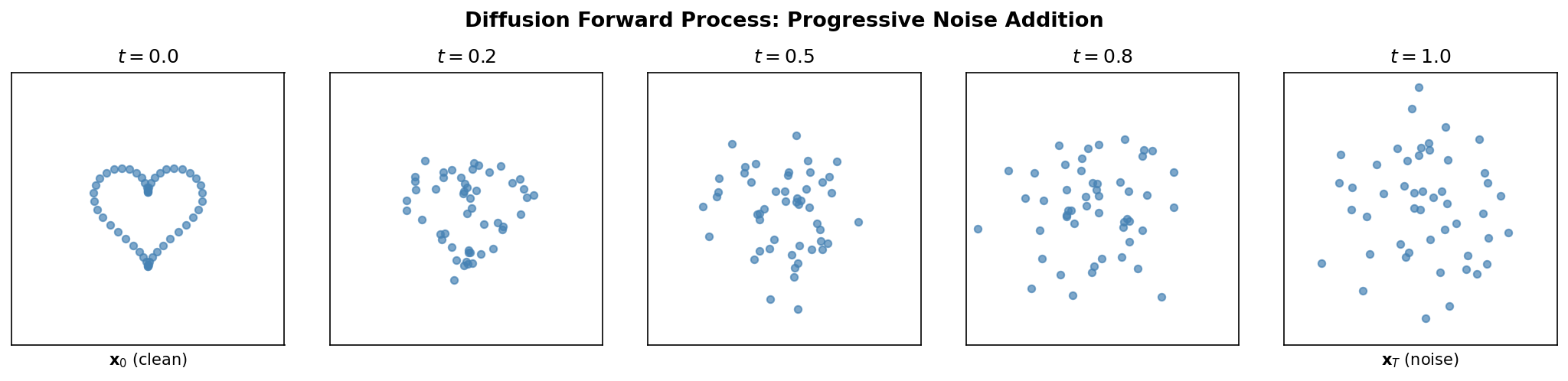
The Forward Process: Adding Noise
Let \(x_0\) denote a clean data point—say, the 3D coordinates of a protein backbone or a continuous embedding of a sequence. The forward process produces a sequence of increasingly noisy versions \(x_1, x_2, \ldots, x_T\) by adding Gaussian noise at each step:
\[q(x_t \mid x_{t-1}) = \mathcal{N}\!\bigl(x_t;\; \sqrt{1 - \beta_t}\, x_{t-1},\; \beta_t I\bigr)\]Here \(\beta_t \in (0, 1)\) is a scalar controlling how much noise is added at step \(t\), and \(T\) is the total number of steps (typically 1000). The collection \(\{\beta_1, \beta_2, \ldots, \beta_T\}\) is called the noise schedule. It usually starts small (gentle corruption early on) and increases over time (aggressive corruption later).
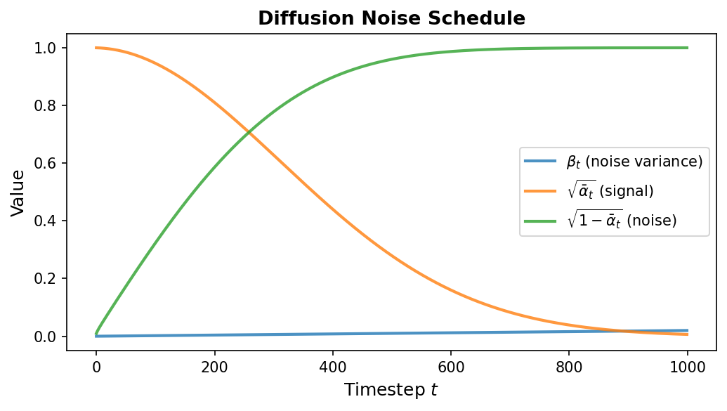
A key mathematical property eliminates the need to apply noise sequentially. Define \(\alpha_t = 1 - \beta_t\) and \(\bar{\alpha}_t = \prod_{s=1}^{t} \alpha_s\) (the cumulative product). Then we can jump directly from \(x_0\) to any \(x_t\):
\[q(x_t \mid x_0) = \mathcal{N}\!\bigl(x_t;\; \sqrt{\bar{\alpha}_t}\, x_0,\; (1 - \bar{\alpha}_t) I\bigr)\]Equivalently:
\[x_t = \sqrt{\bar{\alpha}_t}\, x_0 + \sqrt{1 - \bar{\alpha}_t}\, \epsilon, \quad \epsilon \sim \mathcal{N}(0, I)\]This closed-form expression is essential for efficient training—we can sample any noisy version of the data in a single operation without iterating through all previous timesteps.
class DiffusionSchedule:
    """Precomputes noise schedule quantities for efficient training."""

    def __init__(self, T: int = 1000, beta_start: float = 1e-4,
                 beta_end: float = 0.02):
        self.T = T

        # Linear schedule from beta_start to beta_end
        self.betas = torch.linspace(beta_start, beta_end, T)

        # Precompute alpha, cumulative alpha, and their square roots
        self.alphas = 1.0 - self.betas
        self.alpha_bars = torch.cumprod(self.alphas, dim=0)
        self.sqrt_alpha_bars = torch.sqrt(self.alpha_bars)
        self.sqrt_one_minus_alpha_bars = torch.sqrt(1.0 - self.alpha_bars)

    def add_noise(self, x0: torch.Tensor, t: torch.Tensor,
                  noise: torch.Tensor = None) -> torch.Tensor:
        """Sample x_t from q(x_t | x_0) using the closed-form expression.

        Args:
            x0: clean data, shape [batch, ...]
            t: timestep indices, shape [batch]
            noise: optional pre-sampled noise (same shape as x0)
        """
        if noise is None:
            noise = torch.randn_like(x0)

        # Reshape for broadcasting: [batch, 1, 1, ...]
        sqrt_ab = self.sqrt_alpha_bars[t].view(-1, *([1] * (x0.dim() - 1)))
        sqrt_1m_ab = self.sqrt_one_minus_alpha_bars[t].view(-1, *([1] * (x0.dim() - 1)))

        return sqrt_ab * x0 + sqrt_1m_ab * noise
7. The Reverse Process and Training Objective
Learning to Denoise
The forward process is fixed—no learnable parameters. All the learning happens in the reverse process, which starts from pure noise \(x_T \sim \mathcal{N}(0, I)\) and iteratively recovers the data. Each reverse step is modeled as:
\[p_\theta(x_{t-1} \mid x_t) = \mathcal{N}\!\bigl(x_{t-1};\; \mu_\theta(x_t, t),\; \sigma_t^2 I\bigr)\]where \(\mu_\theta\) is a neural network with parameters \(\theta\) that predicts the denoised mean, and \(\sigma_t^2\) is typically set to \(\beta_t\) (or a related fixed quantity).
Noise Prediction Parameterization
The reverse process requires choosing what quantity the neural network should predict. Three equivalent parameterizations exist: the network can predict the clean data \(x_0\), the posterior mean \(\mu_\theta\), or the noise \(\epsilon\). Ho et al. (2020) found that predicting the noise leads to the simplest and most stable training.
Rather than predicting the mean \(\mu_\theta\) directly, we train the network to predict the noise \(\epsilon\) that was added to obtain \(x_t\) from \(x_0\). Once the network predicts \(\epsilon_\theta(x_t, t)\), we can recover the mean via:
\[\mu_\theta(x_t, t) = \frac{1}{\sqrt{\alpha_t}} \left( x_t - \frac{\beta_t}{\sqrt{1 - \bar{\alpha}_t}}\, \epsilon_\theta(x_t, t) \right)\]The Simple Training Objective
The training loss is the mean squared error between the true noise and the predicted noise, averaged over random timesteps and random noise draws:
\[\mathcal{L}_{\text{simple}} = \mathbb{E}_{t,\, x_0,\, \epsilon}\!\left[\lVert \epsilon - \epsilon_\theta(x_t, t) \rVert^2\right]\]The training procedure for a single batch is:
- Draw a batch of clean data \(x_0\).
- Sample random timesteps \(t \sim \mathrm{Uniform}\{1, \ldots, T\}\).
- Sample random noise \(\epsilon \sim \mathcal{N}(0, I)\).
- Compute noisy data \(x_t = \sqrt{\bar{\alpha}_t}\, x_0 + \sqrt{1 - \bar{\alpha}_t}\, \epsilon\).
- Predict \(\hat{\epsilon} = \epsilon_\theta(x_t, t)\).
- Minimize \(\lVert \epsilon - \hat{\epsilon} \rVert^2\).
def diffusion_training_loss(model: nn.Module, x0: torch.Tensor,
                            schedule: DiffusionSchedule) -> torch.Tensor:
    """Compute the simplified diffusion training loss (noise prediction MSE).

    Args:
        model: noise prediction network, takes (x_t, t) -> predicted noise
        x0: clean data batch, shape [batch, ...]
        schedule: DiffusionSchedule with precomputed quantities
    """
    batch_size = x0.size(0)

    # Step 1: sample random timesteps for each example
    t = torch.randint(0, schedule.T, (batch_size,), device=x0.device)

    # Step 2: sample Gaussian noise
    noise = torch.randn_like(x0)

    # Step 3: compute noisy version x_t
    x_t = schedule.add_noise(x0, t, noise)

    # Step 4: predict the noise
    noise_pred = model(x_t, t)

    # Step 5: MSE between true and predicted noise
    return nn.functional.mse_loss(noise_pred, noise)
This objective has a deep connection to denoising score matching6. The score function \(\nabla_{x} \log p(x)\) points in the direction of increasing data density. Predicting the noise \(\epsilon\) is mathematically equivalent to estimating the score at timestep \(t\), up to a scaling factor. This connection links diffusion models to the broader framework of score-based generative modeling (Song and Ermon, 2019).
8. The Denoising Loop and Network Architecture
Generation by Iterative Denoising
flowchart LR
    XT["x_T\n(pure noise)"] --> D1["Denoise\nStep T"]
    D1 --> XTM["x_{T-1}"] --> D2["Denoise\nStep T-1"]
    D2 --> DOTS["..."]
    DOTS --> D3["Denoise\nStep 1"]
    D3 --> X0["x_0\n(generated\nprotein)"]

    subgraph Step["Each Denoising Step"]
        direction TB
        IN["x_t, t"] --> NET["Neural Network\nε_θ(x_t, t)"]
        NET --> PRED["Predicted noise ε̂"]
        PRED --> SUB["x_{t-1} = f(x_t, ε̂, t)"]
    end

    style XT fill:#fce4ec,stroke:#e91e63
    style X0 fill:#e8f5e9,stroke:#4CAF50
Once the noise prediction network is trained, generation proceeds by simulating the reverse process. Starting from pure noise \(x_T \sim \mathcal{N}(0, I)\), we apply the learned denoising step \(T\) times:
@torch.no_grad()
def ddpm_sample(model: nn.Module, schedule: DiffusionSchedule,
                shape: tuple, device: str = "cpu") -> torch.Tensor:
    """Generate samples via DDPM reverse process.

    Args:
        model: trained noise prediction network
        schedule: DiffusionSchedule with precomputed quantities
        shape: desired output shape, e.g. (n_samples, n_residues, 3)
        device: torch device
    """
    # Start from pure Gaussian noise
    x = torch.randn(shape, device=device)

    for t in reversed(range(schedule.T)):
        t_batch = torch.full((shape[0],), t, device=device, dtype=torch.long)

        # Predict the noise component
        noise_pred = model(x, t_batch)

        # Retrieve schedule quantities for this timestep
        alpha = schedule.alphas[t]
        alpha_bar = schedule.alpha_bars[t]
        beta = schedule.betas[t]

        # Compute the predicted mean of x_{t-1}
        mean = (1.0 / torch.sqrt(alpha)) * (
            x - (beta / torch.sqrt(1.0 - alpha_bar)) * noise_pred
        )

        # Add stochastic noise for all steps except the final one
        if t > 0:
            noise = torch.randn_like(x)
            x = mean + torch.sqrt(beta) * noise
        else:
            x = mean

    return x
At each step except the last (\(t = 0\)), we inject a small amount of fresh noise. This stochasticity ensures diversity: different initial noise samples produce different outputs, and even the same initial noise can yield slightly different results due to the injected randomness during denoising.
Timestep Conditioning
The noise prediction network must know which timestep it is operating at. A heavily corrupted input (\(t\) near \(T\)) requires aggressive denoising, while a lightly corrupted input (\(t\) near 0) needs only gentle refinement. The standard approach borrows sinusoidal position embeddings from the transformer literature to encode the scalar timestep \(t\) as a high-dimensional vector:
import math

class SinusoidalTimestepEmbedding(nn.Module):
    """Encodes scalar timestep t into a d-dimensional vector.

    Uses the same sinusoidal scheme as transformer positional encodings.
    """

    def __init__(self, dim: int):
        super().__init__()
        self.dim = dim

    def forward(self, t: torch.Tensor) -> torch.Tensor:
        device = t.device
        half = self.dim // 2
        freqs = torch.exp(
            -math.log(10000.0) * torch.arange(half, device=device) / half
        )
        args = t[:, None].float() * freqs[None, :]
        return torch.cat([torch.sin(args), torch.cos(args)], dim=-1)
This embedding is then injected into the denoising network—for example, by adding it to intermediate feature maps or concatenating it with the input.
Architecture Choices for Proteins
The choice of denoising network architecture depends on the data representation.
For coordinate-based representations (3D backbone atoms), U-Net architectures with skip connections are common. The encoder half progressively reduces spatial resolution, capturing long-range context, while the decoder half restores resolution. Skip connections from encoder to decoder preserve fine-grained spatial details that would otherwise be lost during downsampling.
For sequence-based representations, transformer architectures work well because attention allows every position to interact with every other position, capturing the long-range dependencies that characterize protein sequences (as discussed in Lecture 1).
In RFDiffusion (Watson et al., 2023), the denoising network is derived from RoseTTAFold, a protein structure prediction model. This is a powerful design choice: the network begins with a deep prior over what realistic protein structures look like, learned from hundreds of thousands of experimentally determined structures. Rather than learning protein physics from scratch, it learns only to denoise—a much easier task when the network already understands structural plausibility.
9. Handling Discrete Protein Data
Diffusion models were designed for continuous data—Gaussian noise added to real-valued vectors. But protein sequences are discrete: each position is one of 20 amino acids (plus possible gap or special tokens). This creates a fundamental mismatch. Three strategies have emerged to address it.
Continuous relaxation. Embed each discrete token into a continuous vector (for instance, using a learned embedding table), apply standard Gaussian diffusion in embedding space, and project back to the nearest discrete token at the end of generation. This is simple to implement but the projection step can introduce artifacts, since the denoised continuous vector may not lie cleanly near any token embedding.
Discrete diffusion (D3PM). Austin et al. (2021) defined corruption processes directly over discrete tokens, where each token transitions to other tokens according to a learned transition matrix rather than Gaussian noise.
Structure-based diffusion. When the goal is to generate protein structures rather than sequences, we can work directly with 3D backbone coordinates, which are naturally continuous. The sequence can then be designed from the generated structure using an inverse folding model such as ProteinMPNN7. This is the strategy used by RFDiffusion.
10. VAEs vs. Diffusion: Choosing the Right Tool
Both VAEs and diffusion models are principled approaches to learning the distribution over proteins. They differ in architecture, training, generation speed, and sample quality. The table below summarizes the key trade-offs.
| Aspect | VAE | Diffusion |
|---|---|---|
| Latent space | Low-dimensional, explicitly structured | Same dimensionality as data; no explicit latent space |
| Training | Single forward pass per example | Multiple noise levels sampled per example |
| Sampling speed | Fast—one decoder pass | Slow—hundreds to thousands of denoising steps |
| Sample quality | Good; can be blurry or mode-averaged | State-of-the-art; captures fine-grained detail |
| Diversity | High | Very high |
| Controllability | Latent-space manipulation, conditional decoding | Classifier guidance, classifier-free guidance |
| Interpretability | Latent dimensions can align with meaningful properties | Less interpretable |
When to prefer a VAE. VAEs are the natural choice when you need a structured latent space for downstream tasks: interpolating between protein families, clustering sequences by function, or optimizing latent vectors with respect to a predicted property. Sampling is cheap (a single decoder forward pass), which matters when screening millions of candidates.
When to prefer diffusion. Diffusion models produce the highest-quality samples available today. When you need physically plausible protein backbones—correct bond lengths, realistic torsion angles, proper secondary-structure packing—diffusion’s iterative refinement outperforms single-shot decoding. The cost is generation time: producing one sample may require 50 to 1000 sequential network evaluations.
Practical hybrid approaches are also common. Latent diffusion models (Rombach et al., 2022) first train a VAE to learn a compressed representation, then apply a diffusion model in the latent space. This combines the structured compression of VAEs with the high sample quality of diffusion, while reducing the computational cost of generation (since diffusion operates in the lower-dimensional latent space rather than the full data space).
A note on computational cost. Generating one protein backbone with RFDiffusion requires roughly 50 denoising steps, each involving a forward pass through a large transformer. On a modern GPU, this takes seconds to minutes depending on protein length. By contrast, a VAE decoder produces a sequence in a single forward pass—milliseconds. For large-scale virtual screening campaigns where millions of candidates must be evaluated, the VAE’s speed advantage is decisive. For targeted design where a few hundred high-quality candidates suffice, diffusion’s superior sample quality justifies the extra compute.
11. Real-World Impact: From Theory to Therapeutics
RFDiffusion: Designing Protein Structures from Scratch
RFDiffusion (Watson et al., 2023) is arguably the most impactful application of diffusion to protein science. Developed by the Baker laboratory at the University of Washington, it generates entirely new protein backbone structures conditioned on diverse design constraints.
The model operates in structure space, diffusing over the 3D coordinates and orientations (rigid-body frames) of protein backbone residues. Starting from random coordinates, it iteratively denoises to produce physically plausible structures. The denoising network is built on RoseTTAFold, a structure prediction architecture, so it carries a deep prior over what realistic protein structures look like.
RFDiffusion has been used to design:
- Novel protein binders for therapeutic targets, including viral surface proteins
- Symmetric protein assemblies—rings, cages, and icosahedral shells
- Proteins with specified topologies and fold geometries
- Enzyme scaffolds with precisely positioned active-site residues
We will study RFDiffusion in depth in Lecture 5, focusing on its SE(3)-equivariant diffusion formulation and its rigid-body frame representation.
EvoDiff: Generating Sequences with Evolutionary Awareness
While RFDiffusion works on structures, EvoDiff (Alamdari et al., 2023) applies diffusion directly to protein sequences using a discrete diffusion framework. Developed at Microsoft Research, it generates sequences that respect the evolutionary patterns learned from millions of natural proteins.
EvoDiff supports several generation modes:
- Unconditional generation: sampling entirely new sequences from the learned distribution
- Family-conditional generation: generating sequences belonging to a specified protein family
- Inpainting: filling in missing or masked regions of a partial sequence
Experimentally, EvoDiff-generated sequences fold into stable structures (as predicted by AlphaFold) and exhibit evolutionary-like conservation patterns, suggesting the model has captured deep structural and functional constraints from sequence data alone.
Conditional Generation: Designing with Intent
The true power of generative models for protein engineering lies in conditional generation—steering the model toward proteins with specific desired properties.
Conditional VAE. The simplest approach conditions the decoder on a property vector (for example, desired thermostability, catalytic activity, or secondary-structure content). The latent code captures sequence variation that is orthogonal to the conditioning signal, enabling diverse generation within a property-defined subspace.
class ConditionalProteinVAE(ProteinVAE):
    """Protein VAE conditioned on a property vector (e.g., stability, function).

    The decoder receives both the latent code z and a learned embedding
    of the condition, enabling property-guided sequence generation.
    """

    def __init__(self, seq_len: int, vocab_size: int = 21,
                 hidden_dim: int = 256, latent_dim: int = 32,
                 condition_dim: int = 10):
        super().__init__(seq_len, vocab_size, hidden_dim, latent_dim)

        # Embed the condition into hidden_dim for concatenation with z
        self.cond_embed = nn.Linear(condition_dim, hidden_dim)

        # Rebuild decoder to accept z + condition embedding
        self.decoder = nn.Sequential(
            nn.Linear(latent_dim + hidden_dim, hidden_dim),
            nn.ReLU(),
            nn.Linear(hidden_dim, seq_len * vocab_size)
        )

    def decode(self, z: torch.Tensor, condition: torch.Tensor):
        """Decode z into amino-acid logits, conditioned on a property vector."""
        cond_emb = self.cond_embed(condition)
        z_cond = torch.cat([z, cond_emb], dim=-1)
        h = self.decoder(z_cond)
        return h.view(-1, self.seq_len, self.vocab_size)
Classifier guidance for diffusion. Dhariwal and Nichol (2021) introduced classifier guidance, where a separately trained classifier steers the denoising process toward a target class. At each denoising step, the gradient of the classifier’s log-probability with respect to the noisy input is added to the predicted denoising direction, pushing the sample toward regions that the classifier associates with the desired property.
@torch.no_grad()
def classifier_guided_sample(
    model: nn.Module,
    classifier: nn.Module,
    schedule: DiffusionSchedule,
    shape: tuple,
    target_class: int,
    guidance_scale: float = 1.0,
    device: str = "cpu"
) -> torch.Tensor:
    """Generate samples steered toward a target class using classifier guidance.

    Args:
        model: trained noise prediction network
        classifier: trained classifier that maps (x_t, t) -> class logits
        schedule: DiffusionSchedule
        shape: desired output shape
        target_class: index of the desired property class
        guidance_scale: strength of guidance (higher = stronger steering)
        device: torch device
    """
    x = torch.randn(shape, device=device)

    for t in reversed(range(schedule.T)):
        t_batch = torch.full((shape[0],), t, device=device, dtype=torch.long)

        # Compute classifier gradient toward target class
        with torch.enable_grad():
            x_grad = x.detach().requires_grad_(True)
            logits = classifier(x_grad, t_batch)
            log_prob = torch.log_softmax(logits, dim=-1)[:, target_class]
            grad = torch.autograd.grad(log_prob.sum(), x_grad)[0]

        # Predict noise, shifted by classifier gradient
        noise_pred = model(x, t_batch)
        noise_pred = noise_pred - guidance_scale * torch.sqrt(
            1.0 - schedule.alpha_bars[t]
        ) * grad

        # Standard DDPM update with the guided noise prediction
        alpha = schedule.alphas[t]
        alpha_bar = schedule.alpha_bars[t]
        beta = schedule.betas[t]

        mean = (1.0 / torch.sqrt(alpha)) * (
            x - (beta / torch.sqrt(1.0 - alpha_bar)) * noise_pred
        )

        if t > 0:
            x = mean + torch.sqrt(beta) * torch.randn_like(x)
        else:
            x = mean

    return x
Classifier-free guidance (Ho and Salimans, 2022) eliminates the need for a separate classifier. During training, the conditioning signal is randomly dropped with some probability, and the model learns both conditional and unconditional generation. At inference time, the conditional and unconditional predictions are blended:
\[\hat{\epsilon} = \epsilon_\theta(x_t, t, \varnothing) + s \cdot \bigl(\epsilon_\theta(x_t, t, c) - \epsilon_\theta(x_t, t, \varnothing)\bigr)\]where \(c\) is the condition, \(\varnothing\) denotes the null condition, and \(s > 1\) amplifies the effect of conditioning. This approach is simpler and often more effective than classifier guidance.
Summary
This lecture covered two foundational frameworks for generative modeling, each with distinct strengths for protein design.
Variational autoencoders learn a probabilistic, low-dimensional latent space. The ELBO training objective balances reconstruction fidelity against latent-space regularity (via the KL divergence). The reparameterization trick makes end-to-end training through stochastic sampling possible. Generation is fast—a single decoder pass—and the structured latent space enables interpolation, clustering, and property-guided optimization.
Diffusion models learn to reverse a gradual noise-corruption process. The forward process has a closed-form expression for any timestep, enabling efficient training. The reverse process is learned by predicting the noise added at each step. Generation requires many sequential denoising steps but produces state-of-the-art sample quality.
For protein science, both frameworks have demonstrated real-world impact. RFDiffusion generates novel protein backbones by diffusing over 3D coordinates. EvoDiff generates evolutionarily plausible sequences via discrete diffusion. Conditional generation—through latent-space conditioning, classifier guidance, or classifier-free guidance—enables designing proteins with targeted properties.
The choice between VAEs and diffusion depends on the application. When you need a fast, interpretable generative model with a structured latent space, choose a VAE. When you need the highest possible sample quality and can tolerate slower generation, choose diffusion. When you want both, consider latent diffusion, which applies diffusion in a VAE’s latent space.
References
- Kingma, D. P. and Welling, M. (2014). “Auto-Encoding Variational Bayes.” International Conference on Learning Representations (ICLR).
- Ho, J., Jain, A., and Abbeel, P. (2020). “Denoising Diffusion Probabilistic Models.” Advances in Neural Information Processing Systems (NeurIPS).
- Watson, J. L. et al. (2023). “De novo design of protein structure and function with RFdiffusion.” Nature, 620, 1089–1100.
- Alamdari, S. et al. (2023). “Protein generation with evolutionary diffusion: sequence is all you need.” Nature Machine Intelligence.
- Austin, J. et al. (2021). “Structured Denoising Diffusion Models in Discrete State-Spaces.” Advances in Neural Information Processing Systems (NeurIPS).
- Higgins, I. et al. (2017). “beta-VAE: Learning Basic Visual Concepts with a Constrained Variational Framework.” International Conference on Learning Representations (ICLR).
- Song, Y. and Ermon, S. (2019). “Generative Modeling by Estimating Gradients of the Data Distribution.” Advances in Neural Information Processing Systems (NeurIPS).
- Dhariwal, P. and Nichol, A. (2021). “Diffusion Models Beat GANs on Image Synthesis.” Advances in Neural Information Processing Systems (NeurIPS).
- Ho, J. and Salimans, T. (2022). “Classifier-Free Diffusion Guidance.” arXiv preprint arXiv:2207.12598.
- Rombach, R. et al. (2022). “High-Resolution Image Synthesis with Latent Diffusion Models.” Conference on Computer Vision and Pattern Recognition (CVPR).
- Dauparas, J. et al. (2022). “Robust deep learning-based protein sequence design using ProteinMPNN.” Science, 378(6615), 49–56.
Exercises
-
Implement and visualize a protein VAE. Train a VAE on a family of homologous protein sequences (for example, from the Pfam database). Project the learned latent codes into 2D using t-SNE or UMAP and color them by subfamily. Do functionally similar sequences cluster together? What happens to the clusters as you increase \(\beta\) from 0.1 to 10?
-
Explore the reconstruction–regularization trade-off. For the VAE trained in Exercise 1, plot reconstruction accuracy (per-position amino-acid recovery rate) and KL divergence as a function of \(\beta\). At what value of \(\beta\) does the latent space become “smooth enough” for generation without destroying reconstruction?
-
Diffusion on a 1D signal. Implement DDPM training and sampling for a simple 1D dataset: per-residue hydrophobicity profiles of real proteins. Visualize the denoising trajectory by plotting \(x_t\) at timesteps \(t \in \{T, 0.75T, 0.5T, 0.25T, 0\}\). How does the structure of the signal emerge over time?
-
Compare VAE and diffusion sample quality. Generate 1000 sequences from a trained VAE and 1000 from a trained diffusion model (using the same training set of protein sequences). Evaluate the naturalness of each set using ESMFold’s pLDDT score or ESM-2 pseudo-perplexity. Which method produces more “protein-like” sequences? How does generation time compare?
-
Conditional protein generation. Extend the
ConditionalProteinVAEabove to condition on a three-element vector representing the target secondary-structure composition (fraction helix, fraction sheet, fraction coil). Train on a dataset where these labels are computed from known structures. Can the model generate sequences that, when folded by ESMFold, match the requested composition within 10 percentage points? -
Discrete vs. continuous diffusion (conceptual). Explain in your own words why adding Gaussian noise to a one-hot-encoded amino-acid sequence does not produce a meaningful corrupted sequence. Describe two strategies for resolving this mismatch and discuss one advantage and one disadvantage of each.
-
The latent code is also called the latent representation, latent variable, or embedding, depending on the community. ↩
-
In Bayesian terminology, the posterior is the distribution over latent variables given observed data. The word “approximate” reminds us that \(q_\phi\) is a parametric family (here, diagonal Gaussians) that may not perfectly match the true posterior. ↩
-
This is called marginal because we integrate (marginalize) over the latent variable \(z\). ↩
-
Jensen’s inequality states that for a concave function \(f\), we have \(f(\mathbb{E}[X]) \geq \mathbb{E}[f(X)]\). Applying it with \(f = \log\) yields the ELBO. ↩
-
The KL divergence \(D_{\mathrm{KL}}(q \,\|\, p) = \int q(z) \log \frac{q(z)}{p(z)}\, dz\) measures how different two distributions are. It is always non-negative and equals zero only when \(q = p\). ↩
-
The score of a distribution \(p(x)\) is the gradient of its log-density, \(\nabla_x \log p(x)\). Score matching trains a network to approximate this gradient without knowing the normalizing constant of \(p\). ↩
-
ProteinMPNN (Dauparas et al., 2022) is a message-passing neural network that predicts amino-acid sequences conditioned on a given protein backbone structure. It is covered in detail in Lecture 6 of this course. ↩