Introduction to AI and Deep Learning
This is Preliminary Note 2 for the Protein & Artificial Intelligence course (Spring 2026), co-taught by Prof. Sungsoo Ahn and Prof. Homin Kim at KAIST. It is designed as a self-study resource: biology-background students should be able to work through it independently before the first in-class lecture. No prior machine learning experience is assumed beyond the material in Preliminary Notes 0 and 1.
Introduction
Imagine you have cloned a gene, designed a construct, and transformed E. coli cells. After overnight expression you lyse the cells, spin down the debris, and pipette off the soluble fraction — only to find that your target protein is trapped in insoluble inclusion bodies. You have just wasted days of bench time. Now imagine a computer program that, given nothing but the amino acid sequence of your construct, predicts with high accuracy whether the protein will be soluble. Building that program is a machine learning problem, and understanding how to solve it is the goal of this note.
We will walk through every concept needed to go from a raw protein sequence to a trained neural network that makes useful predictions. The journey covers five main topics: the machine learning pipeline, the PyTorch tensor library, automatic differentiation, neural network construction, and the training process. We end with a complete case study — predicting protein solubility — that ties every piece together.
Roadmap
The table below maps each section to the specific skill it provides and explains why that skill matters for protein AI.
| Section | Topic | Why You Need It |
|---|---|---|
| 1 | The Machine Learning Pipeline | Provides the big picture: how raw protein data becomes a trained model |
| 2 | PyTorch Tensors | Tensors are the data structure that stores every protein feature, every weight, and every gradient |
| 3 | Automatic Differentiation | Enables neural networks to learn by computing gradients without manual calculus |
| 4 | Building Neural Networks | Teaches you how to assemble layers into architectures suited to protein tasks |
| 5 | Training Neural Networks | Covers loss functions, optimizers, and the training loop that turns data into knowledge |
| 6 | Data Loading | Handles batching, shuffling, and variable-length protein sequences efficiently |
| 7 | Case Study: Protein Solubility | Integrates all concepts into a realistic, end-to-end protein classification project |
| 8 | Best Practices | Practical tips for debugging, reproducibility, and faster training |
Prerequisites
This note builds on two earlier preliminary notes:
- Preliminary Note 0 (Python & Data Basics): NumPy arrays, Pandas DataFrames, FASTA and PDB file parsing.
- Preliminary Note 1 (Protein Representations): One-hot encoding, physicochemical features, distance matrices, and graph representations.
You should also be comfortable with basic linear algebra: vectors, matrices, and matrix multiplication. If the expression \(\mathbf{y} = \mathbf{W}\mathbf{x} + \mathbf{b}\) looks unfamiliar, review the linear algebra appendix in Goodfellow et al. [1] before continuing.
1. The Machine Learning Pipeline
What Does “Learning” Mean for a Computer?
When a biochemist gains experience, they develop intuitions — perhaps that highly charged proteins tend to be soluble, or that long hydrophobic stretches spell trouble. These intuitions are patterns extracted from years of experimental observation. Machine learning does the same thing, but with numbers instead of intuition.
A machine learning model “learns” when it discovers numerical patterns in data that allow it to make accurate predictions on examples it has never seen before. The model does not understand biology the way a scientist does. Instead, it encodes statistical regularities — amino acid composition biases, charge distributions, hydrophobicity patterns — as numerical weights that transform an input protein into a prediction.
The Six Stages
Every machine learning project follows a structured pipeline, as illustrated below.
flowchart LR
    A["📊 Data\nCollection"] --> B["🔧 Preprocessing"]
    B --> C["🧬 Feature\nEngineering"]
    C --> D["🧠 Model\nTraining"]
    D --> E["📏 Evaluation"]
    E --> F["🚀 Deployment"]

    D -->|"Predictions vs Labels"| L["Loss\nFunction"]
    L -->|"Gradients"| U["Parameter\nUpdate"]
    U -->|"Iterate"| D

    style A fill:#e8f4fd,stroke:#2196F3
    style D fill:#fff3e0,stroke:#FF9800
    style F fill:#e8f5e9,stroke:#4CAF50
Each stage presents challenges specific to protein data.
Stage 1: Data Collection. Gather proteins and their associated labels. For solubility prediction, this might mean mining databases like UniProt1 for experimentally validated soluble proteins, or analyzing high-throughput expression studies. The quality of the data fundamentally limits what any model can learn.
Stage 2: Preprocessing. Transform raw data into a clean, consistent format. Protein sequences may contain ambiguous amino acid codes (B for Asp or Asn, X for unknown) or unusual characters that need removal. Structure data from the PDB requires validation for missing atoms, alternate conformations, and resolution quality.
Stage 3: Feature Engineering. This is where domain knowledge meets machine learning. As we explored in Preliminary Note 1, proteins can be represented as one-hot encodings, physicochemical feature vectors, learned embeddings, or graphs. The choice of representation profoundly affects what patterns a model can discover.
Stage 4: Model Training. The model sees thousands of proteins with known labels and gradually adjusts its internal parameters to minimize prediction errors. This stage involves critical choices about model architecture, optimization algorithm, and regularization strategy.
Stage 5: Evaluation. Measure how well the model generalizes to new proteins. This is trickier than it sounds. Related sequences often have similar properties, so a naive random train/test split might let the model “cheat” by memorizing similar proteins. Proper evaluation requires sequence-identity-aware splitting2 to ensure the test set contains truly novel proteins.
Stage 6: Deployment. Bring the model into production where it makes predictions on new proteins. Practical constraints around inference speed, memory usage, and integration with existing laboratory workflows become important here.
Flavors of Machine Learning
Different biological questions call for different learning strategies.
Supervised learning is the most straightforward flavor. You have input-output pairs — protein sequences and their solubility labels, structures and their stability measurements — and you want to learn the mapping between them. The key requirement is labeled data, which in biology often comes from expensive experiments.
Unsupervised learning works without labels. Instead, it discovers structure in the data itself: clustering similar protein sequences, learning low-dimensional embeddings that capture evolutionary relationships, or identifying protein families. Unsupervised learning can leverage the vast quantities of unlabeled sequence data in databases like UniProt.
Self-supervised learning has revolutionized protein machine learning in recent years. The idea is to create supervision signals from the data itself. For example, mask out 15% of amino acids in a protein sequence and train the model to predict the missing residues. This task, borrowed from natural language processing3, forces the model to learn deep representations of protein sequence-structure-function relationships. Models like ESM [4] and ProtTrans [5], trained on hundreds of millions of protein sequences with this approach, have become foundational tools in computational biology.
Matching Problems to Formulations
Different biological questions map to different mathematical formulations. Getting this mapping right is the first step in any project.
Regression problems have continuous outputs. Predicting a protein’s melting temperature (\(T_m\)) or dissociation constant (\(K_d\)) are regression tasks. The model outputs a real number, and we measure error as the difference between prediction and ground truth.
Binary classification distinguishes two categories. Is this protein an enzyme or not? Will it be soluble when expressed in E. coli? The model outputs a probability between 0 and 1, and we apply a threshold to make a decision.
Multi-class classification extends binary classification to more than two categories. Predicting which of several secondary structure states each residue adopts, or classifying proteins into major functional categories, are examples.
Multi-label classification handles cases where multiple labels can apply to the same protein simultaneously. A protein might be both an enzyme and membrane-bound. Each label is predicted independently.
Sequence-to-sequence tasks produce one output per input position. Secondary structure prediction assigns one of three states (helix, sheet, coil) to every residue. Disorder prediction identifies which residues lack fixed three-dimensional structure.
2. PyTorch: Your Laboratory for Neural Networks
If machine learning is the science, PyTorch is the laboratory equipment. Just as a biochemist needs pipettes, centrifuges, and spectrophotometers, a computational biologist needs tools for constructing and training neural networks. PyTorch, developed by Meta AI Research [2], has become the dominant framework for deep learning research, including the models that have transformed protein science.
Three properties make PyTorch the standard choice. First, its “eager execution” model means code runs line by line, making debugging straightforward. Second, its design closely mirrors how researchers think about computation, so translating mathematical ideas into working code is natural. Third, the entire ecosystem of protein AI — from ESM to OpenFold — builds on PyTorch.
Tensors: The Atoms of Deep Learning
At the heart of PyTorch lies the tensor, a multi-dimensional array of numbers. If you have used NumPy arrays (Preliminary Note 0), tensors will feel familiar.
A single number is a 0-dimensional tensor, called a scalar. A list of numbers is a 1-dimensional tensor, called a vector. A table of numbers is a 2-dimensional tensor, called a matrix. Higher dimensions are common in practice: a batch of protein sequences might be stored as a 3-dimensional tensor with shape (batch_size, sequence_length, features).
import torch

# --- Creating tensors ---
# A 3x4 matrix of zeros (e.g., placeholder for 3 proteins with 4 features)
x = torch.zeros(3, 4)

# A 3x4 matrix of ones
x = torch.ones(3, 4)

# Random values from a standard normal distribution (mean=0, std=1)
x = torch.randn(3, 4)

# From a Python list (e.g., hydrophobicity values for three amino acids)
x = torch.tensor([1.8, -4.5, 2.5])

# From a NumPy array (bridge between NumPy and PyTorch)
import numpy as np
np_array = np.array([[1.0, 2.0], [3.0, 4.0]])
x = torch.from_numpy(np_array)

# --- Inspecting tensor properties ---
x = torch.randn(3, 4)
print(x.shape)   # torch.Size([3, 4]) — the dimensions
print(x.dtype)   # torch.float32 — the numerical precision
print(x.device)  # cpu — where the tensor lives (cpu or cuda:0)
What makes tensors special compared to NumPy arrays? Two things: GPU acceleration and automatic differentiation.
The GPU Advantage
Modern GPUs (Graphics Processing Units) contain thousands of simple processors that perform arithmetic operations in parallel. A single NVIDIA GPU can execute trillions of floating-point operations per second. This massive parallelism is well suited to the matrix multiplications at the heart of neural networks.
Moving computation to the GPU requires just one line in PyTorch:
# Check whether a GPU is available on this machine
device = torch.device('cuda' if torch.cuda.is_available() else 'cpu')
print(f"Using device: {device}")

# Create a tensor on the CPU, then move it to the GPU
x = torch.randn(1000, 1000)
x_gpu = x.to(device)

# Matrix multiplication now runs on the GPU
y_gpu = x_gpu @ x_gpu.T
For a 1000-by-1000 matrix multiplication, a GPU can be 50–100 times faster than a CPU. When training neural networks that involve millions of such operations per second, this speedup is the difference between experiments taking hours versus weeks.
Tensor Operations
Tensors support all the arithmetic you would expect, with the same broadcasting rules4 as NumPy.
a = torch.randn(3, 4)
b = torch.randn(3, 4)

# Element-wise operations (applied independently to each pair of elements)
c = a + b          # Addition
c = a * b          # Multiplication (element-wise, NOT matrix multiplication)
c = a ** 2         # Square each element

# Matrix multiplication (the workhorse of neural networks)
# A 3x4 matrix times a 4x3 matrix produces a 3x3 matrix
c = a @ b.T                   # @ is the matrix multiplication operator
c = torch.matmul(a, b.T)     # Equivalent, more explicit

# Broadcasting: a smaller tensor is "stretched" to match
a = torch.randn(3, 4)   # Shape: (3, 4)
b = torch.randn(4)      # Shape: (4,)
c = a + b               # b is broadcast across all 3 rows → shape (3, 4)

# Reductions: summarize a tensor along one or more dimensions
x = torch.randn(3, 4)
x.sum()           # Sum of all 12 elements → a scalar
x.sum(dim=0)      # Sum along rows → shape (4,)
x.mean(dim=-1)    # Mean along the last dimension → shape (3,)
x.max(dim=1)      # Maximum along columns → returns (values, indices)
Reshaping: The Art of Tensor Origami
Neural networks constantly reshape data as it flows through layers. A batch of protein sequences might start as shape (batch, length, 20) for one-hot encodings, then become (batch, 128, length) after an embedding layer with 128 features. Mastering reshaping is essential.
x = torch.randn(2, 3, 4)  # 2 batches, 3 positions, 4 features

# view / reshape: change dimensions while preserving the total number of elements
# 2*3 = 6 rows, 4 columns
x.view(6, 4)
x.reshape(2, 12)     # Flatten the last two dims: 3*4 = 12

# transpose: swap two specific dimensions
x.transpose(0, 1)    # Swap dim 0 and dim 1 → shape (3, 2, 4)

# permute: reorder all dimensions at once
x.permute(2, 0, 1)   # New order: features, batch, positions → shape (4, 2, 3)

# unsqueeze / squeeze: add or remove dimensions of size 1
x.unsqueeze(0)        # Add a dimension at position 0 → shape (1, 2, 3, 4)
x.squeeze()           # Remove all size-1 dimensions
A common use case: PyTorch’s 1D convolution layers (nn.Conv1d) expect input of shape (batch, channels, length), but protein sequence data is often stored as (batch, length, channels). A single .transpose(1, 2) fixes this mismatch.
3. Automatic Differentiation: Teaching Computers Calculus
How does a neural network learn? The answer involves calculus — but not the tedious symbol manipulation you may recall from introductory courses. Neural networks learn through an algorithmic trick called automatic differentiation (often shortened to autograd).
The Intuition Behind Learning
Suppose you are trying to predict protein solubility. Your model takes a protein sequence as input and outputs a number between 0 and 1, representing the predicted probability of being soluble. For a protein you know to be soluble (true label \(y = 1\)), if the model predicts \(\hat{y} = 0.3\), it is wrong.
We quantify this “wrongness” with a loss function — a single number that measures the gap between prediction and reality. A simple choice is squared error: \((y - \hat{y})^2 = (1 - 0.3)^2 = 0.49\).
Now comes the key insight. Your model’s prediction depends on its internal parameters, called weights. Different weight values produce different predictions. Some weight values would push the prediction closer to 1 (reducing the loss), while others would make it worse. Learning means finding weight values that minimize the loss across all training proteins.
Gradients Point Downhill
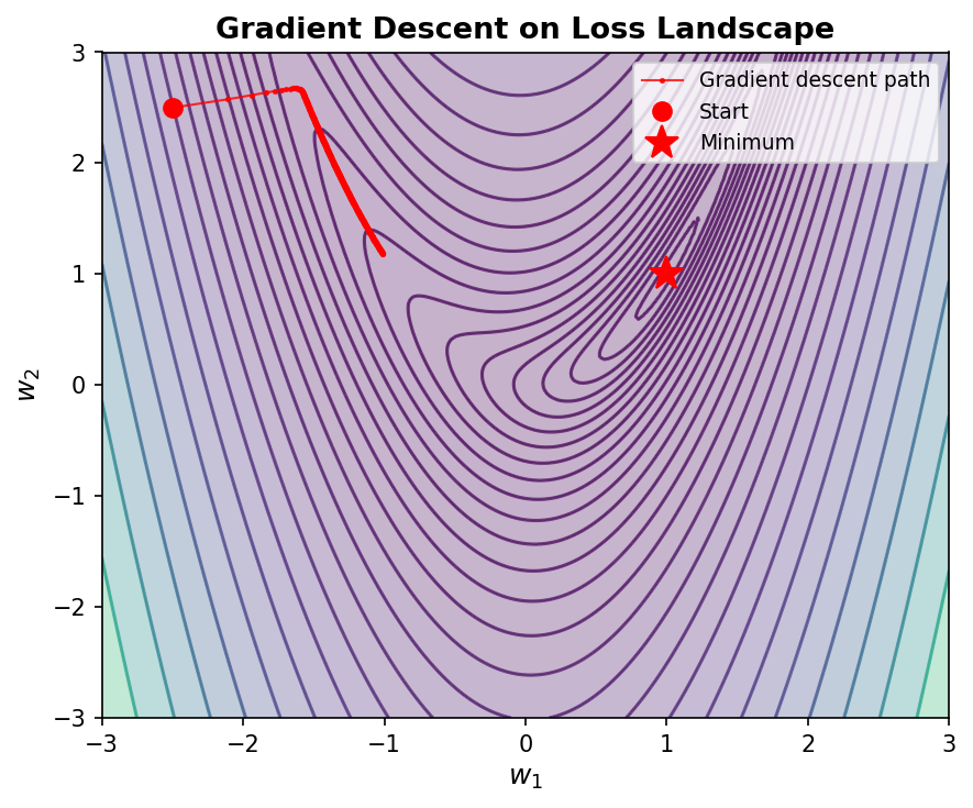
How do we find good weight values? We use gradients. The gradient of the loss with respect to a weight tells us: “if I increase this weight by a tiny amount, how does the loss change?”
- If increasing a weight would increase the loss, we should decrease that weight.
- If increasing a weight would decrease the loss, we should increase it.
This strategy — adjusting each weight in the direction that reduces the loss — is called gradient descent5.
The Chain Rule: Propagating Blame
A neural network composes many simple functions: the output of one layer feeds into the next, which feeds into the next. To compute how a weight in an early layer affects the final loss, we need the chain rule from calculus.
Let \(x\) be the input to some function that produces \(y\), and let \(L\) be the loss computed from \(y\). The chain rule states:
\[\frac{\partial L}{\partial x} = \frac{\partial L}{\partial y} \cdot \frac{\partial y}{\partial x}\]In words: to find how \(x\) affects \(L\), multiply how \(y\) affects \(L\) by how \(x\) affects \(y\). Applied recursively backward through the network — from the loss, through each layer, all the way to the first weight — this gives us gradients for every parameter. This recursive backward application of the chain rule is the backpropagation algorithm6.
The following diagram shows a simple computation graph and how gradients flow backward through it during backpropagation.
flowchart LR
    subgraph Forward["Forward Pass →"]
        x["x"] -->|"×W"| z["z = Wx + b"]
        b["b"] -->|"+b"| z
        z -->|"σ(·)"| a["a = σ(z)"]
        a -->|"L(·)"| L["Loss L"]
    end

    subgraph Backward["← Backward Pass"]
        dL["∂L/∂L = 1"] -->|"∂L/∂a"| da["∂L/∂a"]
        da -->|"∂a/∂z = σ'(z)"| dz["∂L/∂z"]
        dz -->|"∂z/∂W = x"| dW["∂L/∂W"]
        dz -->|"∂z/∂b = 1"| db["∂L/∂b"]
    end

    style Forward fill:#e8f4fd,stroke:#2196F3
    style Backward fill:#fce4ec,stroke:#e91e63
PyTorch Autograd in Action
The remarkable thing about PyTorch is that you never need to implement backpropagation yourself. You define only the forward computation — how inputs become outputs. PyTorch automatically builds a computational graph that tracks every operation. When you call .backward(), it traverses this graph in reverse, computing all gradients.
# Create a tensor and tell PyTorch to track operations on it
x = torch.tensor([2.0, 3.0], requires_grad=True)

# Forward computation: y_i = x_i^2 + 3*x_i
y = x ** 2 + 3 * x

# The loss must be a scalar (single number) for .backward()
z = y.sum()

# Backward pass: compute dz/dx for each element of x
z.backward()

# Gradients are stored in the .grad attribute
print(x.grad)  # tensor([7., 9.])
Let us verify this by hand. We have \(z = \sum_i (x_i^2 + 3x_i)\), so the partial derivative is \(\frac{\partial z}{\partial x_i} = 2x_i + 3\). For \(x_1 = 2\): \(2(2) + 3 = 7\). For \(x_2 = 3\): \(2(3) + 3 = 9\). PyTorch computed exactly these values — automatically.
A More Realistic Example: Linear Regression
Here is a scenario closer to real protein modeling. Suppose we have 100 proteins, each described by 10 physicochemical features, and we want to predict a continuous property (say, melting temperature). We model the relationship as a linear function: \(\hat{y} = \mathbf{X}\mathbf{W} + b\), where \(\mathbf{X}\) is the feature matrix, \(\mathbf{W}\) is a weight vector, and \(b\) is a bias term.
# Simulated data: 100 proteins, 10 features each
X = torch.randn(100, 10)   # Feature matrix
y = torch.randn(100, 1)    # True melting temperatures (simulated)

# Learnable parameters — requires_grad=True is crucial!
W = torch.randn(10, 1, requires_grad=True)   # Weight vector
b = torch.zeros(1, requires_grad=True)        # Bias term

# Forward pass: compute predictions
y_pred = X @ W + b                # Matrix multiply + broadcast bias

# Loss: mean squared error
loss = ((y_pred - y) ** 2).mean()

# Backward pass: compute gradients of loss w.r.t. W and b
loss.backward()

# W.grad now contains dL/dW — the direction to adjust each weight
print(f"Weight gradient shape: {W.grad.shape}")  # torch.Size([10, 1])
print(f"Bias gradient shape:   {b.grad.shape}")   # torch.Size([1])
The gradient W.grad tells us how to nudge each weight to reduce the loss. This is the foundation upon which all neural network training rests.
Turning Off Gradient Tracking
Computing gradients consumes memory (to store the computational graph) and time. During inference — when you just want predictions, not training — you should disable gradient tracking:
# Context manager: temporarily disable gradient tracking
with torch.no_grad():
    y_pred = model(x)
    # No computational graph is built — faster and more memory-efficient

# Decorator: permanently disable gradients inside a function
@torch.no_grad()
def predict(model, x):
    return model(x)
4. Building Neural Networks: From Neurons to Architectures
With tensors for data and autograd for gradients, we can now build neural networks. Let us construct them from the ground up, using protein examples throughout.
The Single Neuron
The fundamental unit is the artificial neuron. It takes multiple inputs, computes a weighted sum, adds a bias, and applies a nonlinear function:
\[\text{output} = \sigma(w_1 x_1 + w_2 x_2 + \cdots + w_n x_n + b)\]Here \(x_1, x_2, \ldots, x_n\) are the input values (for example, the hydrophobicity, charge, and length of a protein). The weights \(w_1, w_2, \ldots, w_n\) determine how much each input contributes. The bias \(b\) shifts the decision boundary. The function \(\sigma\) is called an activation function; it introduces nonlinearity, allowing the neuron to model relationships that are not straight lines.
Two widely used activation functions are:
- ReLU (Rectified Linear Unit): \(\sigma(z) = \max(0, z)\). Simple and effective. Sets negative values to zero and passes positive values unchanged.
- Sigmoid: \(\sigma(z) = \frac{1}{1 + e^{-z}}\). Squashes any input into the range \((0, 1)\), making it useful when the output should represent a probability.
- Softmax: Given a vector \(\mathbf{z}\), \(\text{softmax}(z_i) = \frac{e^{z_i}}{\sum_j e^{z_j}}\). Normalizes a vector of real numbers into a probability distribution that sums to 1. Used in classification (choosing among classes) and in attention mechanisms (computing how much each element should attend to every other).
- GELU (Gaussian Error Linear Unit): \(\text{GELU}(z) = z \cdot \Phi(z)\), where \(\Phi\) is the standard Gaussian cumulative distribution function. A smooth approximation of ReLU that allows small negative values to pass through. Widely used in transformer architectures.
- Swish (also called SiLU): \(\text{Swish}(z) = z \cdot \sigma(z)\), where \(\sigma\) is the sigmoid function. Like GELU, it is smooth and non-monotonic. Used in ESM-2 and other recent protein models.
Layers: Many Neurons in Parallel
A single neuron is limited. But arrange many neurons in parallel — each receiving the same inputs but with different weights — and you get a layer. With 64 neurons, you get 64 different weighted combinations of the input features. This can be written compactly as a matrix equation:
\[\mathbf{h} = \sigma(\mathbf{W}\mathbf{x} + \mathbf{b})\]where \(\mathbf{W}\) is a weight matrix of shape (64, n_inputs), \(\mathbf{x}\) is the input vector, \(\mathbf{b}\) is a bias vector, and \(\mathbf{h}\) is the output vector of 64 values. This is a fully connected layer (also called a dense layer or linear layer).
Depth: Stacking Layers
flowchart LR
    subgraph Input["Input Layer"]
        I1["x₁\n(hydrophob.)"]
        I2["x₂\n(charge)"]
        I3["x₃\n(length)"]
    end

    subgraph Hidden1["Hidden Layer 1\n(64 neurons)"]
        H1["h₁"]
        H2["h₂"]
        H3["..."]
        H4["h₆₄"]
    end

    subgraph Hidden2["Hidden Layer 2\n(32 neurons)"]
        G1["g₁"]
        G2["g₂"]
        G3["..."]
        G4["g₃₂"]
    end

    subgraph Output["Output Layer"]
        O1["ŷ₁\n(soluble)"]
        O2["ŷ₂\n(insoluble)"]
    end

    I1 & I2 & I3 --> H1 & H2 & H3 & H4
    H1 & H2 & H3 & H4 --> G1 & G2 & G3 & G4
    G1 & G2 & G3 & G4 --> O1 & O2

    style Input fill:#e8f4fd,stroke:#2196F3
    style Hidden1 fill:#fff3e0,stroke:#FF9800
    style Hidden2 fill:#fff3e0,stroke:#FF9800
    style Output fill:#e8f5e9,stroke:#4CAF50
The power of neural networks comes from stacking multiple layers. The output of one layer becomes the input to the next. Each successive layer can learn increasingly abstract representations of the input.
For a protein property classifier, this hierarchy might look like:
- Layer 1 detects individual amino acid properties (charge, size, hydrophobicity).
- Layer 2 recognizes local motifs (charge clusters, hydrophobic patches).
- Layer 3 identifies higher-order patterns (domain boundaries, structural elements).
- Output layer combines these abstract representations into a final prediction.
This hierarchical learning is what makes deep learning “deep.” The depth allows the network to build complex features from simple ones, much like how protein structure emerges from local interactions at the residue level.
nn.Module: PyTorch’s Building Block
In PyTorch, every neural network component inherits from nn.Module. This base class provides machinery for tracking parameters, moving to GPU, saving and loading models, and more. Building a custom network means writing a class with two methods:
-
__init__: define what layers exist. -
forward: define how data flows through them.
import torch.nn as nn

class ProteinNet(nn.Module):
    """A simple feedforward network for protein property prediction."""

    def __init__(self, input_dim, hidden_dim, output_dim):
        super().__init__()
        # First fully connected layer: input features → hidden representation
        self.fc1 = nn.Linear(input_dim, hidden_dim)
        # Activation function
        self.relu = nn.ReLU()
        # Second fully connected layer: hidden representation → prediction
        self.fc2 = nn.Linear(hidden_dim, output_dim)

    def forward(self, x):
        # x shape: (batch_size, input_dim)
        x = self.fc1(x)    # Linear transformation
        x = self.relu(x)   # Nonlinear activation
        x = self.fc2(x)    # Map to output
        return x

# Create the model: 20 amino acid features → 64 hidden units → 2 classes
model = ProteinNet(input_dim=20, hidden_dim=64, output_dim=2)

# Use the model: pass a batch of 32 proteins, each with 20 features
x = torch.randn(32, 20)
output = model(x)         # Shape: (32, 2)
print(output.shape)
PyTorch handles the backward pass automatically. You never write backpropagation code — you only specify the forward computation.
Common Layer Types
PyTorch provides a library of pre-built layers for common operations. Here are the ones you will encounter most often in protein AI.
# --- Linear layer ---
# Computes y = Wx + b. The fundamental building block.
nn.Linear(in_features=20, out_features=64)

# --- Activation functions ---
nn.ReLU()        # max(0, x) — simple, effective, the default choice
nn.GELU()        # Smooth approximation of ReLU, used in transformer models
nn.Sigmoid()     # Squashes output to (0, 1), useful for binary probabilities
nn.Softmax(dim=-1)  # Normalizes a vector to sum to 1 (probability distribution)

# --- Normalization layers ---
# Stabilize training by normalizing intermediate activations
nn.LayerNorm(normalized_shape=64)    # Normalizes across features (used in transformers)
nn.BatchNorm1d(num_features=64)      # Normalizes across the batch dimension

# --- Dropout ---
# Randomly zeros out neurons during training to prevent overfitting
nn.Dropout(p=0.1)  # Each neuron has a 10% chance of being turned off per forward pass

# --- Embedding layer ---
# Maps discrete tokens (like amino acid indices) to continuous vectors
# 21 possible tokens (20 amino acids + 1 padding), each mapped to a 64-dim vector
nn.Embedding(num_embeddings=21, embedding_dim=64)
nn.Sequential: Quick Model Definition
For simple architectures where data flows straight through one layer after another with no branching, nn.Sequential offers a compact shortcut:
model = nn.Sequential(
    nn.Linear(20, 64),     # 20 input features → 64 hidden units
    nn.ReLU(),
    nn.Dropout(0.1),       # Regularization
    nn.Linear(64, 64),     # Second hidden layer
    nn.ReLU(),
    nn.Dropout(0.1),
    nn.Linear(64, 2)       # Output: 2 classes (soluble vs. insoluble)
)
This builds the same network as a custom nn.Module class but with less boilerplate. Use nn.Sequential for quick experiments; switch to a full class when you need branching, skip connections, or conditional logic.
Managing Parameters
Neural networks can have millions of parameters. PyTorch provides tools to inspect and manage them.
# List all named parameters and their shapes
for name, param in model.named_parameters():
    print(f"{name}: shape={param.shape}, requires_grad={param.requires_grad}")

# Count total and trainable parameters
total_params = sum(p.numel() for p in model.parameters())
trainable_params = sum(p.numel() for p in model.parameters() if p.requires_grad)
print(f"Total parameters:     {total_params:,}")
print(f"Trainable parameters: {trainable_params:,}")

# Save a trained model's weights to disk
torch.save(model.state_dict(), 'protein_model.pt')

# Load weights back into a model (the architecture must match)
model.load_state_dict(torch.load('protein_model.pt'))
5. Training Neural Networks: The Learning Loop
Training a neural network is an iterative process. You show the model examples, measure its mistakes, compute the direction of improvement, and nudge the weights accordingly. This section covers each component of this process in detail.
Loss Functions: Measuring Mistakes
Before the model can learn, we need a way to quantify how wrong its predictions are. The loss function (also called a cost function or objective function) produces a single number: zero means perfect predictions, and larger values mean worse predictions.
Different problem types require different loss functions.
Mean Squared Error (MSE)
MSE is the standard loss for regression tasks — predicting continuous values like binding affinity or melting temperature. Let \(y_i\) be the true value and \(\hat{y}_i\) be the predicted value for protein \(i\), with \(n\) proteins in total:
\[\text{MSE} = \frac{1}{n}\sum_{i=1}^{n}(y_i - \hat{y}_i)^2\]Squaring the error penalizes large mistakes heavily. A prediction that is off by 10 degrees contributes 100 to the sum, while one that is off by 1 degree contributes only 1.
Binary Cross-Entropy (BCE)
BCE is designed for binary classification — tasks with two categories, such as soluble versus insoluble. Let \(y_i \in \{0, 1\}\) be the true label and \(\hat{y}_i \in (0, 1)\) be the predicted probability:
\[\text{BCE} = -\frac{1}{n}\sum_{i=1}^{n}\bigl[y_i \log(\hat{y}_i) + (1 - y_i)\log(1 - \hat{y}_i)\bigr]\]The intuition: when the true label is 1, we want \(\hat{y}_i\) close to 1, making \(\log(\hat{y}_i)\) close to 0 (low loss). When the true label is 0, we want \(\hat{y}_i\) close to 0, making \(\log(1 - \hat{y}_i)\) close to 0.
Cross-Entropy (CE)
CE generalizes BCE to multi-class classification — tasks with more than two categories. Let \(C\) be the number of classes, \(y_c \in \{0, 1\}\) be the indicator for class \(c\), and \(\hat{y}_c\) be the predicted probability for class \(c\):
\[\text{CE} = -\sum_{c=1}^{C} y_c \log(\hat{y}_c)\]In practice, only one \(y_c\) is 1 (the true class), so this simplifies to \(-\log(\hat{y}_{\text{true class}})\).
In PyTorch:
# Regression: predict melting temperature
criterion = nn.MSELoss()

# Binary classification: soluble vs. insoluble
# BCEWithLogitsLoss combines sigmoid + BCE for numerical stability
criterion = nn.BCEWithLogitsLoss()

# Multi-class classification: predict secondary structure (H, E, C)
# CrossEntropyLoss combines softmax + CE for numerical stability
criterion = nn.CrossEntropyLoss()
Optimizers: Choosing a Learning Strategy
The loss function tells us how wrong we are. The optimizer tells us how to improve. It takes the gradients computed by backpropagation and uses them to update the weights.
Stochastic Gradient Descent (SGD)
SGD is the simplest optimizer. Update each weight by taking a step in the direction that reduces the loss:
\[\theta_{t+1} = \theta_t - \eta \nabla_\theta L\]Here \(\theta_t\) represents the current weight values, \(\eta\) is the learning rate (a small positive number controlling step size), and \(\nabla_\theta L\) is the gradient of the loss with respect to the weights.
The learning rate is one of the most important hyperparameters7 in training. Too small, and learning is painfully slow. Too large, and training becomes unstable — the loss oscillates wildly or diverges to infinity.
Adam: Adaptive Moment Estimation
Adam [3] is the most popular optimizer in practice. It maintains two running averages for each weight: the mean of recent gradients (\(m_t\), the “first moment”) and the mean of recent squared gradients (\(v_t\), the “second moment”). These allow it to adapt the learning rate individually for each parameter:
\[m_t = \beta_1 m_{t-1} + (1 - \beta_1) g_t\] \[v_t = \beta_2 v_{t-1} + (1 - \beta_2) g_t^2\] \[\theta_{t+1} = \theta_t - \eta \frac{m_t}{\sqrt{v_t} + \epsilon}\]Here \(g_t\) is the gradient at step \(t\), \(\beta_1\) and \(\beta_2\) are decay rates (typically 0.9 and 0.999), and \(\epsilon\) is a small constant for numerical stability (typically \(10^{-8}\)).
The intuition: parameters with consistently large gradients take smaller steps (the denominator \(\sqrt{v_t}\) is large), while parameters with small or noisy gradients take larger steps. This adaptive behavior makes Adam work well out of the box for most problems.
# SGD with momentum (momentum helps smooth out noisy gradient estimates)
optimizer = torch.optim.SGD(model.parameters(), lr=0.01, momentum=0.9)

# Adam — the default choice for most protein AI projects
optimizer = torch.optim.Adam(model.parameters(), lr=1e-3)

# AdamW — Adam with decoupled weight decay (better regularization)
optimizer = torch.optim.AdamW(model.parameters(), lr=1e-4, weight_decay=0.01)
The Training Loop: Four Steps, Repeated
Training unfolds as a repeated cycle of four steps. Each iteration of this cycle processes one batch of training examples (a subset of the full dataset). One pass through the entire dataset is called an epoch.
Step 1: Forward pass. Feed a batch of proteins through the model to produce predictions. Data flows forward through the network, layer by layer.
Step 2: Compute loss. Compare predictions to true labels using the loss function. This produces a single scalar measuring how wrong we are on this batch.
Step 3: Backward pass. Call loss.backward() to compute gradients for all parameters. Each gradient answers: “how should this weight change to reduce the loss?”
Step 4: Update weights. The optimizer uses the gradients to adjust the weights. We have now learned from this batch.
def train_one_epoch(model, dataloader, criterion, optimizer, device):
    """Train the model for one pass through the dataset."""
    model.train()   # Enable training mode (activates dropout, etc.)
    total_loss = 0

    for batch_x, batch_y in dataloader:
        # Move data to the same device as the model (CPU or GPU)
        batch_x = batch_x.to(device)
        batch_y = batch_y.to(device)

        # Step 1: Forward pass — compute predictions
        predictions = model(batch_x)

        # Step 2: Compute loss — measure prediction error
        loss = criterion(predictions, batch_y)

        # Step 3: Backward pass — compute gradients
        optimizer.zero_grad()   # Clear gradients from the previous batch!
        loss.backward()         # Compute new gradients

        # Optional: clip gradients to prevent exploding values
        torch.nn.utils.clip_grad_norm_(model.parameters(), max_norm=1.0)

        # Step 4: Update weights — apply gradient descent
        optimizer.step()

        total_loss += loss.item()   # .item() extracts a Python float

    avg_loss = total_loss / len(dataloader)
    return avg_loss
A critical detail: optimizer.zero_grad() must be called before each backward pass. By default, PyTorch accumulates gradients — calling .backward() multiple times adds to the existing .grad values rather than replacing them. Without zeroing, gradients from previous batches would contaminate the current update8.
Validation: Detecting Overfitting
Training loss alone can be misleading. A model might memorize the training examples perfectly (achieving near-zero training loss) without learning patterns that generalize to new proteins. This is called overfitting.
To detect overfitting, we evaluate the model on a separate validation set that it never trains on:
@torch.no_grad()   # No gradient computation needed during evaluation
def evaluate(model, dataloader, criterion, device):
    """Evaluate the model on a held-out dataset."""
    model.eval()    # Disable dropout, use running statistics for batch norm
    total_loss = 0
    all_predictions = []
    all_labels = []

    for batch_x, batch_y in dataloader:
        batch_x = batch_x.to(device)
        batch_y = batch_y.to(device)

        predictions = model(batch_x)
        loss = criterion(predictions, batch_y)

        total_loss += loss.item()
        all_predictions.append(predictions.cpu())
        all_labels.append(batch_y.cpu())

    avg_loss = total_loss / len(dataloader)
    all_predictions = torch.cat(all_predictions)
    all_labels = torch.cat(all_labels)

    return avg_loss, all_predictions, all_labels
The pattern is clear: if training loss decreases but validation loss increases, the model is overfitting. The best model is the one with the lowest validation loss, not the lowest training loss.
Putting It All Together: A Complete Training Script
A production-quality training script adds two important techniques:
- Learning rate scheduling: gradually reduce the learning rate as training progresses, allowing finer adjustments near a good solution.
- Early stopping: halt training when validation loss stops improving, preventing wasted computation and overfitting.
def train_model(model, train_loader, val_loader, epochs=100, patience=10):
    """Full training pipeline with learning rate scheduling and early stopping."""
    device = torch.device('cuda' if torch.cuda.is_available() else 'cpu')
    model = model.to(device)

    criterion = nn.CrossEntropyLoss()
    optimizer = torch.optim.Adam(model.parameters(), lr=1e-3)

    # Reduce learning rate by half when validation loss stops improving for 5 epochs
    scheduler = torch.optim.lr_scheduler.ReduceLROnPlateau(
        optimizer, mode='min', patience=5, factor=0.5
    )

    best_val_loss = float('inf')
    patience_counter = 0

    for epoch in range(epochs):
        # --- Training phase ---
        train_loss = train_one_epoch(model, train_loader, criterion, optimizer, device)

        # --- Validation phase ---
        val_loss, _, _ = evaluate(model, val_loader, criterion, device)

        # --- Adjust learning rate ---
        scheduler.step(val_loss)

        # --- Early stopping ---
        if val_loss < best_val_loss:
            best_val_loss = val_loss
            patience_counter = 0
            torch.save(model.state_dict(), 'best_model.pt')  # Save the best model
        else:
            patience_counter += 1
            if patience_counter >= patience:
                print(f"Early stopping at epoch {epoch}")
                break

        # --- Logging ---
        current_lr = optimizer.param_groups[0]['lr']
        print(f"Epoch {epoch:3d} | train_loss={train_loss:.4f} | "
              f"val_loss={val_loss:.4f} | lr={current_lr:.6f}")

    # Load the best model before returning
    model.load_state_dict(torch.load('best_model.pt'))
    return model
6. Data Loading: Feeding Proteins to Neural Networks
Training neural networks requires showing them thousands or millions of examples. Efficient data loading becomes crucial, especially when proteins have variable lengths and complex representations.
The Dataset Class
PyTorch’s Dataset class defines how to access individual examples. You implement two methods:
-
__len__: returns the total number of examples. -
__getitem__: returns one example by its index.
Here is a dataset for protein sequences:
from torch.utils.data import Dataset, DataLoader

class ProteinDataset(Dataset):
    """A dataset of protein sequences and their labels."""

    def __init__(self, sequences, labels, max_len=512):
        self.sequences = sequences
        self.labels = labels
        self.max_len = max_len

        # Map each of the 20 standard amino acids to an integer (1–20)
        # Index 0 is reserved for padding
        self.aa_to_idx = {aa: i + 1 for i, aa in enumerate('ACDEFGHIKLMNPQRSTVWY')}

    def __len__(self):
        return len(self.sequences)

    def __getitem__(self, idx):
        seq = self.sequences[idx]
        label = self.labels[idx]

        # Convert amino acid characters to integers
        # Truncate sequences longer than max_len
        encoded = torch.zeros(self.max_len, dtype=torch.long)
        for i, aa in enumerate(seq[:self.max_len]):
            encoded[i] = self.aa_to_idx.get(aa, 0)  # Unknown amino acids → 0

        # Create a mask: 1 for real positions, 0 for padding
        seq_len = min(len(seq), self.max_len)
        mask = torch.zeros(self.max_len, dtype=torch.float)
        mask[:seq_len] = 1.0

        return {
            'sequence': encoded,        # Shape: (max_len,)
            'mask': mask,               # Shape: (max_len,)
            'label': torch.tensor(label, dtype=torch.long)
        }
The DataLoader: Batching and Shuffling
The DataLoader wraps a dataset and handles three important tasks:
- Batching: groups individual examples into batches for efficient GPU computation.
- Shuffling: randomizes the order of examples each epoch so the model does not learn spurious ordering patterns.
- Parallel loading: uses multiple worker processes to prepare the next batch while the GPU trains on the current one.
# Create dataset objects
train_dataset = ProteinDataset(train_sequences, train_labels)
val_dataset = ProteinDataset(val_sequences, val_labels)

# Wrap in DataLoaders
train_loader = DataLoader(
    train_dataset,
    batch_size=32,        # Process 32 proteins at a time
    shuffle=True,         # Randomize order each epoch (important for training)
    num_workers=4,        # Use 4 parallel processes for data loading
    pin_memory=True       # Faster CPU → GPU transfer
)

val_loader = DataLoader(
    val_dataset,
    batch_size=64,        # Larger batches are fine for evaluation (no gradients stored)
    shuffle=False         # Keep a consistent order for reproducible evaluation
)

# Iterate through batches
for batch in train_loader:
    sequences = batch['sequence']   # Shape: (32, max_len)
    masks = batch['mask']           # Shape: (32, max_len)
    labels = batch['label']         # Shape: (32,)
    # ... feed to model ...
Handling Variable-Length Sequences
Proteins range from tens to thousands of amino acids. Padding every sequence to the length of the longest protein in the entire dataset wastes computation and memory. A custom collate function can pad each batch only to its own maximum length:
def collate_proteins(batch):
    """Pad sequences in a batch to the length of the longest sequence in that batch."""
    # Find the maximum length in this specific batch
    max_len = max(len(item['sequence']) for item in batch)

    sequences = torch.zeros(len(batch), max_len, dtype=torch.long)
    masks = torch.zeros(len(batch), max_len)
    labels = torch.zeros(len(batch), dtype=torch.long)

    for i, item in enumerate(batch):
        seq_len = len(item['sequence'])
        sequences[i, :seq_len] = item['sequence']
        masks[i, :seq_len] = 1.0
        labels[i] = item['label']

    return {'sequence': sequences, 'mask': masks, 'label': labels}

# Pass the custom collate function to the DataLoader
loader = DataLoader(dataset, batch_size=32, collate_fn=collate_proteins)
This reduces wasted computation when batches contain only short sequences.
7. Case Study: Predicting Protein Solubility
Let us bring every concept together in a complete, end-to-end application: predicting whether a protein will be soluble when expressed in E. coli.
Why Solubility Prediction Matters
Expressing recombinant proteins is a core technique in structural biology, biotechnology, and therapeutic development. When a target protein aggregates into inclusion bodies instead of dissolving in the cytoplasm, downstream applications — crystallography, assays, drug formulation — become much harder or impossible. A computational model that predicts solubility from sequence alone can guide construct design and save weeks of experimental effort.
What makes this problem amenable to machine learning? Solubility is influenced by sequence-level properties: amino acid composition, charge distribution, hydrophobicity patterns, and the presence of certain sequence motifs. These patterns are learnable from data.
The Model Architecture
We build a 1D convolutional neural network (CNN) that processes amino acid embeddings. The architecture reflects domain knowledge: convolutional layers with a kernel size of 5 can detect patterns spanning five consecutive amino acids, which is appropriate for capturing local sequence motifs like charge clusters or hydrophobic stretches.
import torch.nn.functional as F

class ProteinSolubilityClassifier(nn.Module):
    """
    A 1D-CNN for predicting protein solubility from amino acid sequence.

    Architecture:
    1. Embedding: map each amino acid index to a learned 64-dim vector
    2. Two Conv1d layers: detect local sequence motifs
    3. Global average pooling: aggregate over the full sequence
    4. Linear output: predict soluble (1) vs. insoluble (0)
    """

    def __init__(self, vocab_size=21, embed_dim=64, hidden_dim=128, num_classes=2):
        super().__init__()

        # Embedding layer: integers → continuous vectors
        # padding_idx=0 ensures the padding token always maps to a zero vector
        self.embedding = nn.Embedding(vocab_size, embed_dim, padding_idx=0)

        # 1D convolutions detect local patterns in the sequence
        # kernel_size=5 means each filter looks at 5 consecutive amino acids
        # padding=2 preserves the sequence length after convolution
        self.conv1 = nn.Conv1d(embed_dim, hidden_dim, kernel_size=5, padding=2)
        self.conv2 = nn.Conv1d(hidden_dim, hidden_dim, kernel_size=5, padding=2)

        # Classification head
        self.fc = nn.Linear(hidden_dim, num_classes)
        self.dropout = nn.Dropout(0.3)

    def forward(self, x, mask=None):
        # x shape: (batch, seq_len) — integer-encoded amino acids

        # Step 1: Embed amino acids → (batch, seq_len, embed_dim)
        x = self.embedding(x)

        # Step 2: Rearrange for Conv1d → (batch, embed_dim, seq_len)
        x = x.transpose(1, 2)

        # Step 3: Apply convolutions with ReLU activation
        x = F.relu(self.conv1(x))    # → (batch, hidden_dim, seq_len)
        x = self.dropout(x)
        x = F.relu(self.conv2(x))    # → (batch, hidden_dim, seq_len)

        # Step 4: Global average pooling over the sequence dimension
        # Use the mask to ignore padding positions
        if mask is not None:
            mask = mask.unsqueeze(1)             # → (batch, 1, seq_len)
            x = (x * mask).sum(dim=2) / mask.sum(dim=2).clamp(min=1)
        else:
            x = x.mean(dim=2)                   # → (batch, hidden_dim)

        # Step 5: Classify → (batch, num_classes)
        x = self.fc(x)
        return x
Preparing the Data
from sklearn.model_selection import train_test_split
import pandas as pd

# Load a solubility dataset (e.g., from the SOLpro or eSOL databases)
df = pd.read_csv('solubility_data.csv')
print(f"Dataset size: {len(df)} proteins")
print(f"Class distribution:\n{df['label'].value_counts()}")

# Split into train / validation / test sets
# Stratify by label to maintain class balance in each split
train_df, temp_df = train_test_split(df, test_size=0.2, stratify=df['label'],
                                     random_state=42)
val_df, test_df = train_test_split(temp_df, test_size=0.5, stratify=temp_df['label'],
                                   random_state=42)

print(f"Train: {len(train_df)}, Val: {len(val_df)}, Test: {len(test_df)}")

# Create Dataset and DataLoader objects
train_dataset = ProteinDataset(train_df['sequence'].tolist(),
                               train_df['label'].tolist())
val_dataset = ProteinDataset(val_df['sequence'].tolist(),
                             val_df['label'].tolist())
test_dataset = ProteinDataset(test_df['sequence'].tolist(),
                              test_df['label'].tolist())

train_loader = DataLoader(train_dataset, batch_size=32, shuffle=True)
val_loader = DataLoader(val_dataset, batch_size=64, shuffle=False)
test_loader = DataLoader(test_dataset, batch_size=64, shuffle=False)
Training
# Instantiate the model and inspect its size
model = ProteinSolubilityClassifier()
n_params = sum(p.numel() for p in model.parameters())
print(f"Model parameters: {n_params:,}")

# Train with early stopping and learning rate scheduling
trained_model = train_model(model, train_loader, val_loader, epochs=50, patience=10)
Evaluation: Beyond Accuracy
A single accuracy number rarely tells the full story. For a solubility dataset where 70% of proteins are soluble, a model that always predicts “soluble” achieves 70% accuracy while being completely useless. We need a richer set of metrics.
from sklearn.metrics import (accuracy_score, precision_recall_fscore_support,
                             roc_auc_score)

def evaluate_classifier(model, test_loader, device):
    """Evaluate a binary classifier with multiple metrics."""
    model.eval()
    all_preds = []
    all_labels = []
    all_probs = []

    with torch.no_grad():
        for batch in test_loader:
            x = batch['sequence'].to(device)
            mask = batch['mask'].to(device)
            y = batch['label']

            logits = model(x, mask)                         # Raw scores
            probs = F.softmax(logits, dim=-1)               # Probabilities
            preds = logits.argmax(dim=-1)                   # Predicted class

            all_preds.extend(preds.cpu().numpy())
            all_labels.extend(y.numpy())
            all_probs.extend(probs[:, 1].cpu().numpy())     # P(soluble)

    # Compute metrics
    accuracy = accuracy_score(all_labels, all_preds)
    precision, recall, f1, _ = precision_recall_fscore_support(
        all_labels, all_preds, average='binary'
    )
    auc = roc_auc_score(all_labels, all_probs)

    print(f"Accuracy:  {accuracy:.4f}")
    print(f"Precision: {precision:.4f}")
    print(f"Recall:    {recall:.4f}")
    print(f"F1 Score:  {f1:.4f}")
    print(f"AUC-ROC:   {auc:.4f}")

    return accuracy, precision, recall, f1, auc
Here is what each metric tells you:
| Metric | Question It Answers | When It Matters |
|---|---|---|
| Accuracy | What fraction of all predictions are correct? | Balanced datasets only |
| Precision | Of proteins predicted soluble, what fraction truly are? | When false positives are costly (wasting expression experiments) |
| Recall | Of proteins that are soluble, what fraction did we detect? | When missing a soluble protein is costly (screening large libraries) |
| F1 Score | Harmonic mean of precision and recall | When you care equally about false positives and false negatives |
| AUC-ROC | How well does the model separate classes across all thresholds? | Threshold-independent assessment of overall discriminative power |
8. Best Practices for Deep Learning
Training neural networks involves many subtle decisions. The practices below, drawn from years of community experience, will help you avoid common pitfalls.
Debugging Neural Networks
Neural networks can fail silently. The code runs, the loss decreases, but predictions are useless. Systematic debugging is essential.
# 1. Check for NaN gradients (sign of numerical instability)
for name, param in model.named_parameters():
    if param.grad is not None and torch.isnan(param.grad).any():
        print(f"WARNING: NaN gradient detected in {name}")

# 2. Verify that outputs are in a sensible range
with torch.no_grad():
    sample_output = model(sample_input)
    print(f"Output range: [{sample_output.min():.3f}, {sample_output.max():.3f}]")

# 3. Confirm that input and output shapes match expectations
print(f"Input shape:  {sample_input.shape}")
print(f"Output shape: {model(sample_input).shape}")

# 4. Sanity check: can the model overfit a single batch?
# If it cannot, there is likely a bug in the architecture or loss
small_batch_x, small_batch_y = next(iter(train_loader))
for step in range(200):
    pred = model(small_batch_x.to(device))
    loss = criterion(pred, small_batch_y.to(device))
    optimizer.zero_grad()
    loss.backward()
    optimizer.step()
    if step % 50 == 0:
        print(f"Step {step}: loss = {loss.item():.4f}")
# Loss should approach 0. If it does not, debug your model.
Reproducibility
Science requires reproducibility. Set all random seeds at the start of every experiment:
import random
import numpy as np

def set_seed(seed=42):
    """Set random seeds for reproducibility across all libraries."""
    random.seed(seed)
    np.random.seed(seed)
    torch.manual_seed(seed)
    torch.cuda.manual_seed_all(seed)
    # For full determinism on GPU (may reduce performance slightly):
    torch.backends.cudnn.deterministic = True
    torch.backends.cudnn.benchmark = False

set_seed(42)
Full determinism on GPU can slow training by 10–20%. For exploratory experiments, setting the Python, NumPy, and PyTorch seeds is usually sufficient. Reserve full determinism for final reported results.
Mixed Precision Training
Modern GPUs have specialized hardware for 16-bit floating-point (FP16) arithmetic that runs roughly twice as fast as 32-bit (FP32) operations. Mixed precision training uses FP16 where possible and FP32 where numerical precision is critical (e.g., loss accumulation and weight updates):
from torch.cuda.amp import autocast, GradScaler

scaler = GradScaler()

for batch_x, batch_y in train_loader:
    batch_x = batch_x.to(device)
    batch_y = batch_y.to(device)
    optimizer.zero_grad()

    # Forward pass in FP16 (faster, less memory)
    with autocast():
        predictions = model(batch_x)
        loss = criterion(predictions, batch_y)

    # Backward pass with gradient scaling (prevents FP16 underflow)
    scaler.scale(loss).backward()
    scaler.step(optimizer)
    scaler.update()
Mixed precision typically provides a 1.5–2x speedup with minimal impact on model accuracy. It also reduces GPU memory usage, allowing larger batch sizes.
A Practical Checklist
Before declaring a model “trained,” verify the following:
- Training loss decreases steadily over epochs.
- Validation loss decreases initially, then plateaus (not increases — that signals overfitting).
- The model can perfectly overfit a single batch (sanity check for bugs).
- Gradients are finite (no NaN or Inf values).
- Metrics on the test set are consistent with validation set metrics.
- Results are reproducible when the same seed is used.
Key Takeaways
-
Machine learning discovers patterns in protein data automatically, encoding them as numerical weights that transform sequences into predictions.
-
Tensors are the universal data structure of deep learning. They combine NumPy-like operations with GPU acceleration and automatic differentiation.
-
Autograd implements the chain rule algorithmically, computing gradients for all model parameters from the forward computation alone. You never write backpropagation by hand.
-
Neural networks are compositions of simple layers: linear transformations followed by nonlinear activations. The
nn.Moduleclass provides the framework for building and managing them. -
Training is a four-step loop — forward pass, loss computation, backward pass, weight update — repeated across many epochs. Early stopping and learning rate scheduling are essential for good results.
-
Data loading with
DatasetandDataLoaderhandles batching, shuffling, and parallel processing. Custom collate functions manage variable-length protein sequences efficiently. -
Evaluation must use held-out data and multiple metrics. For proteins, sequence-identity-aware splits prevent data leakage from homologous sequences.
Exercises
These exercises reinforce the concepts from this note. Each one can be completed in a single Python script or Jupyter notebook.
Exercise 1: Per-Residue Secondary Structure Prediction
Build a 3-layer MLP that predicts secondary structure for each residue in a protein sequence. The model should take a one-hot encoded sequence of shape (batch, length, 20) and output three probabilities (helix, sheet, coil) for each position, giving output shape (batch, length, 3).
Hints:
- Use
nn.CrossEntropyLoss()with the input reshaped to(batch * length, 3). - Think carefully about how to handle padding positions in the loss computation.
Exercise 2: Learning Rate Warmup
Modify the training loop to implement linear warmup: start with a very small learning rate (e.g., \(10^{-7}\)) and linearly increase it to the target learning rate (e.g., \(10^{-3}\)) over the first 1,000 training steps.
Hint: Use torch.optim.lr_scheduler.LinearLR or manually adjust optimizer.param_groups[0]['lr'] at each step.
Exercise 3: Gradient Accumulation
Implement gradient accumulation to simulate a batch size of 128 when your GPU can only fit 32 samples at a time. The idea: run four forward/backward passes (each with 32 samples), accumulate the gradients, and then call optimizer.step() once.
Key detail: You should call optimizer.zero_grad() only once per effective batch (every 4 mini-batches), not at every step.
Exercise 4: Optimizer Comparison
Train the ProteinSolubilityClassifier from Section 7 three times, each with a different optimizer:
- SGD with momentum 0.9
- Adam with default settings
- AdamW with weight decay 0.01
Plot the training and validation loss curves for all three on the same graph. Which optimizer converges fastest? Which achieves the lowest final validation loss?
Exercise 5: Custom Metric
Implement Matthews Correlation Coefficient (MCC), a metric that is informative even when classes are severely imbalanced:
\[\text{MCC} = \frac{TP \cdot TN - FP \cdot FN}{\sqrt{(TP + FP)(TP + FN)(TN + FP)(TN + FN)}}\]where \(TP\), \(TN\), \(FP\), and \(FN\) are the counts of true positives, true negatives, false positives, and false negatives respectively. Add this metric to the evaluate_classifier function and compare it to accuracy on a dataset where 90% of proteins are soluble.
References
-
Goodfellow, I., Bengio, Y., & Courville, A. (2016). Deep Learning. MIT Press. Chapters 6–8. Available at https://www.deeplearningbook.org/.
-
Paszke, A., Gross, S., Massa, F., Lerer, A., Bradbury, J., Chanan, G., … & Chintala, S. (2019). “PyTorch: An Imperative Style, High-Performance Deep Learning Library.” Advances in Neural Information Processing Systems, 32.
-
Kingma, D. P. & Ba, J. (2015). “Adam: A Method for Stochastic Optimization.” Proceedings of the 3rd International Conference on Learning Representations (ICLR).
-
Rives, A., Meier, J., Sercu, T., Goyal, S., Lin, Z., Liu, J., … & Fergus, R. (2021). “Biological Structure and Function Emerge from Scaling Unsupervised Learning to 250 Million Protein Sequences.” Proceedings of the National Academy of Sciences, 118(15), e2016239118.
-
Elnaggar, A., Heinzinger, M., Dallago, C., Rehawi, G., Wang, Y., Jones, L., … & Rost, B. (2022). “ProtTrans: Toward Understanding the Language of Life Through Self-Supervised Learning.” IEEE Transactions on Pattern Analysis and Machine Intelligence, 44(10), 7112–7127.
-
Rumelhart, D. E., Hinton, G. E., & Williams, R. J. (1986). “Learning Representations by Back-Propagating Errors.” Nature, 323(6088), 533–536.
-
PyTorch Documentation. https://pytorch.org/docs/stable/.
-
PyTorch Tutorials. https://pytorch.org/tutorials/.
-
UniProt (Universal Protein Resource) is the most comprehensive database of protein sequences and functional annotations, containing over 200 million entries as of 2025. ↩
-
Sequence-identity-aware splitting clusters proteins by sequence similarity (e.g., using CD-HIT at 30% identity) and assigns entire clusters to either train or test, preventing information leakage from homologous sequences. ↩
-
The masked prediction task was popularized by BERT (Bidirectional Encoder Representations from Transformers) in natural language processing. The protein versions of this idea are sometimes called “protein language models.” ↩
-
Broadcasting is a set of rules that allow operations between tensors of different shapes. When two tensors have different numbers of dimensions or different sizes along a dimension, the smaller tensor is “stretched” (conceptually, not in memory) to match the larger one. For example, adding a vector of shape
(4,)to a matrix of shape(3, 4)adds the vector to each row. ↩ -
The term “stochastic gradient descent” (SGD) refers to gradient descent applied to a random subset (mini-batch) of the training data at each step, rather than the entire dataset. In practice, almost all gradient descent in deep learning is stochastic. ↩
-
Backpropagation was popularized for neural network training by Rumelhart, Hinton, and Williams in 1986, though the mathematical idea of reverse-mode automatic differentiation predates it. ↩
-
A hyperparameter is a setting chosen by the practitioner before training begins (like learning rate, batch size, or number of layers), as opposed to a parameter learned during training (like the weights of a linear layer). ↩
-
Gradient accumulation is sometimes used intentionally. When GPU memory is too small for a large batch, you can run several small forward/backward passes, accumulate their gradients, and then call
optimizer.step()once. This simulates training with a larger effective batch size. ↩