Diffusion Models for Protein Generation

This is Lecture 4 of the Protein & Artificial Intelligence course (Spring 2026), co-taught by Prof. Sungsoo Ahn and Prof. Homin Kim at KAIST. It assumes familiarity with variational autoencoders from Lecture 3. All code examples use PyTorch.

Introduction

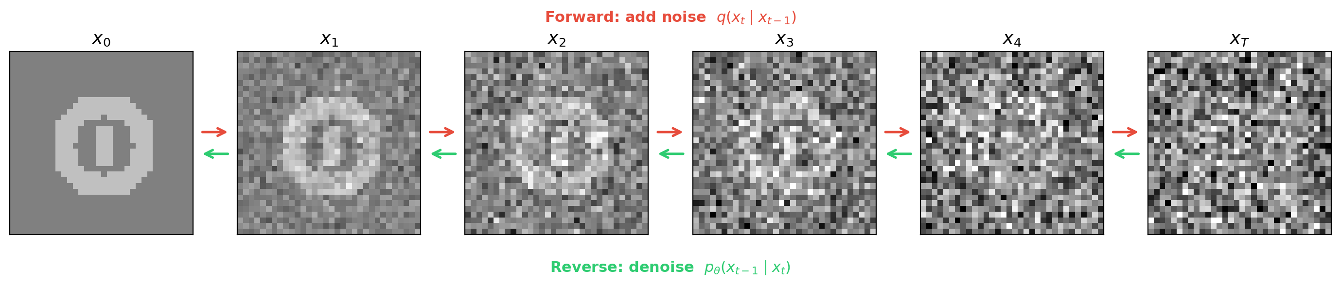
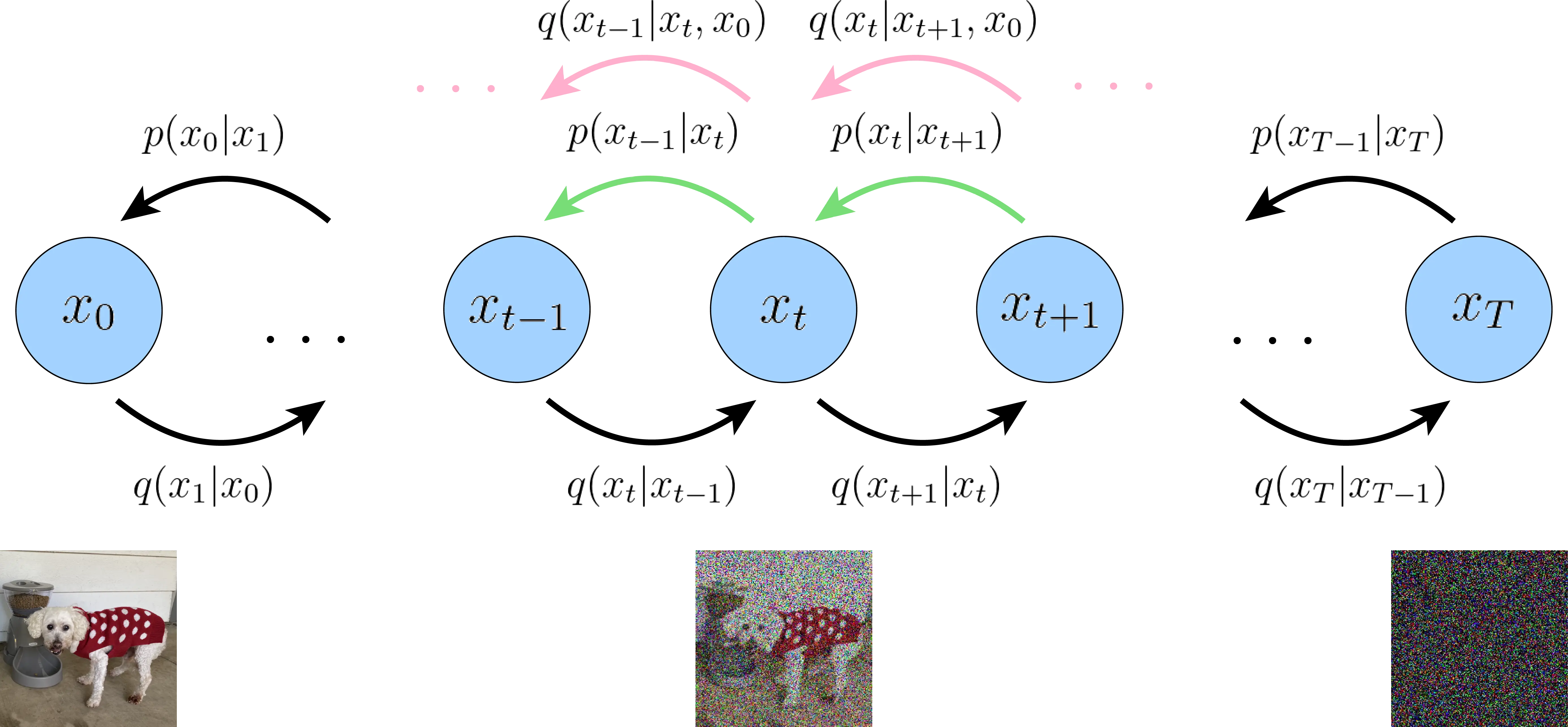
Sharpening a blurry photograph is far easier than painting a photorealistic image from a blank canvas. Diffusion models exploit this asymmetry: instead of generating proteins from scratch, they decompose generation into many small denoising steps—gradually removing noise from random coordinates until a realistic protein backbone emerges.

The same idea applies to any continuous data. Take the 3D coordinates of a protein backbone and jitter every atom by a tiny random displacement. The resulting structure is still recognizable, and a neural network could plausibly predict the original positions from this lightly perturbed version. Repeat the corruption many times until the coordinates become indistinguishable from random points in space. If the network can reverse each individual step, chaining all the reverse steps together recovers a clean structure from pure noise.

This lecture develops denoising diffusion probabilistic models from first principles: the forward noising process, the reverse denoising objective, the connection to score matching, and practical generation. We close by comparing diffusion with VAEs and covering conditional generation—the techniques that steer diffusion models toward specific protein properties.

Roadmap

1. The Forward Process: Controlled Destruction

Diffusion on an image. The forward process \(q\) progressively adds Gaussian noise until the image becomes indistinguishable from random noise. The reverse process \(p_\theta\) learns to undo each step, recovering the clean image from pure noise.

Diffusion on a point cloud. Structured coordinates (left) are progressively corrupted until they resemble a random Gaussian scatter (right). The reverse process learns to recover the original structure step by step. For proteins, the points represent residue positions in 3D space.

Adding Noise

Let \(x_0 \in \mathbb{R}^D\) denote a clean data point—say, the 3D coordinates of a protein backbone or a continuous embedding of a sequence. The forward process produces a sequence of increasingly noisy versions \(x_1, x_2, \ldots, x_T\) by adding Gaussian noise at each step:

Here \(\beta_t \in (0, 1)\) is a scalar controlling how much noise is added at step \(t\), and \(T\) is the total number of steps (typically 1000). The collection \(\{\beta_1, \beta_2, \ldots, \beta_T\}\) is called the noise schedule. It usually starts small (gentle corruption early on) and increases over time (aggressive corruption later).

Forward diffusion process. (a) Three example trajectories: clean data \(x\) (top) is progressively corrupted through noisy versions \(z_{20}, z_{40}, \ldots, z_{100}\), converging to pure noise. (b) The conditional distributions \(q(z_1|x)\), \(q(z_{41}|z_{40})\), \(q(z_{81}|z_{80})\) at selected steps. Each step adds a small amount of Gaussian noise, so the conditional is a narrow Gaussian centered near the previous value. As diffusion progresses, the distributions widen and overlap, erasing information about the starting point. Source: Prince, Understanding Deep Learning, CC BY-NC-ND. Used without modification.

A linear noise schedule over 1000 timesteps. β_t (noise variance per step) increases linearly. √ᾱ_t (signal coefficient) decays from 1 to near 0 — the clean signal is gradually destroyed. √(1−ᾱ_t) (noise coefficient) grows from 0 to 1 — by t=T, the data is pure noise.

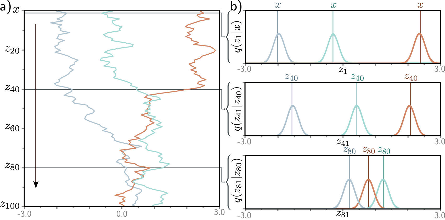
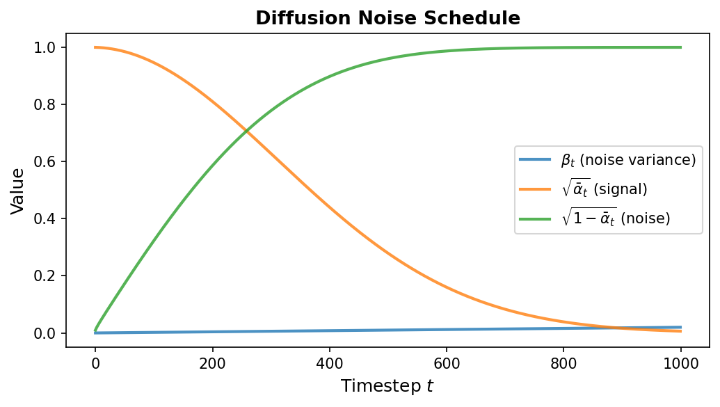
A key mathematical property eliminates the need to apply noise sequentially. Define \(\alpha_t = 1 - \beta_t\) and \(\bar{\alpha}_t = \prod_{s=1}^{t} \alpha_s\) (the cumulative product). Then we can jump directly from \(x_0\) to any \(x_t\):

Equivalently:

This closed-form expression is essential for efficient training—we can sample any noisy version of the data in a single operation without iterating through all previous timesteps.

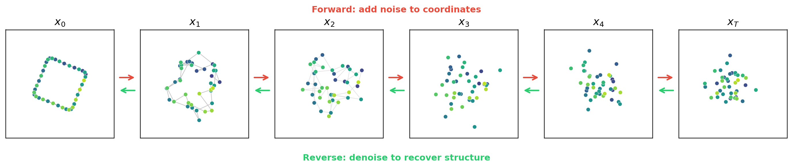
For the bead-spring polymer from Lecture 3, \(x_0 \in \mathbb{R}^{24}\) is the preprocessed coordinate vector (12 beads \(\times\) 2D, center-of-mass subtracted and PCA-aligned). The forward process progressively corrupts the 2D bead positions — a compact coil or extended chain — until they resemble a random scatter of 12 points. Because the data is 24-dimensional (far simpler than images or 3D protein structures), \(T = 200\) steps with a linear schedule from \(\beta_1 = 10^{-4}\) to \(\beta_{200} = 0.02\) suffices.

class DiffusionSchedule:
    """Precomputes noise schedule quantities for efficient training."""

    def __init__(self, T: int = 1000, beta_start: float = 1e-4,
                 beta_end: float = 0.02):
        self.T = T

        # Linear schedule from beta_start to beta_end
        self.betas = torch.linspace(beta_start, beta_end, T)

        # Precompute alpha, cumulative alpha, and their square roots
        self.alphas = 1.0 - self.betas
        self.alpha_bars = torch.cumprod(self.alphas, dim=0)
        self.sqrt_alpha_bars = torch.sqrt(self.alpha_bars)
        self.sqrt_one_minus_alpha_bars = torch.sqrt(1.0 - self.alpha_bars)

    def add_noise(self, x0: torch.Tensor, t: torch.Tensor,
                  noise: torch.Tensor = None) -> torch.Tensor:
        """Sample x_t from q(x_t | x_0) using the closed-form expression.

        Args:
            x0: clean data, shape [batch, ...]
            t: timestep indices, shape [batch]
            noise: optional pre-sampled noise (same shape as x0)
        """
        if noise is None:
            noise = torch.randn_like(x0)

        # Reshape for broadcasting: [batch, 1, 1, ...]
        sqrt_ab = self.sqrt_alpha_bars[t].view(-1, *([1] * (x0.dim() - 1)))
        sqrt_1m_ab = self.sqrt_one_minus_alpha_bars[t].view(-1, *([1] * (x0.dim() - 1)))

        return sqrt_ab * x0 + sqrt_1m_ab * noise

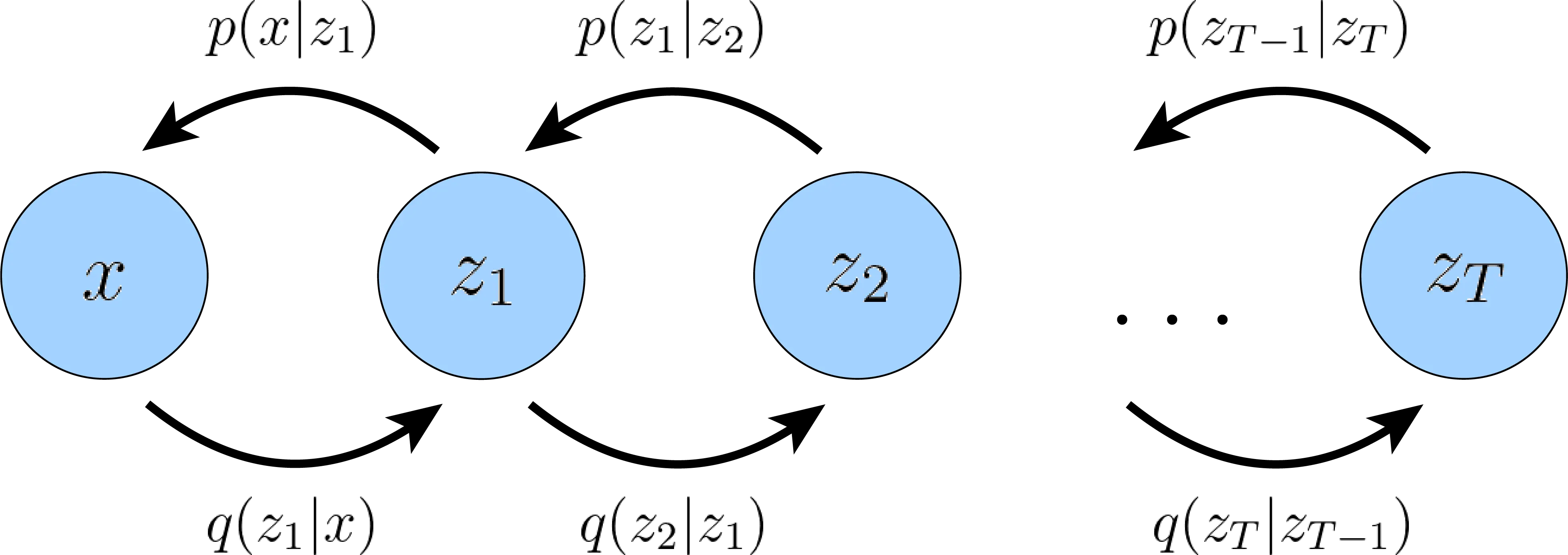
2. The Reverse Process and Training Objective

Learning to Denoise

The forward process is fixed—no learnable parameters. All the learning happens in the reverse process, which starts from pure noise \(x_T \sim \mathcal{N}(0, I)\) and iteratively recovers the data. Each reverse step is modeled as:

where \(\mu_\theta\) is a neural network with parameters \(\theta\) that predicts the denoised mean, and \(\sigma_t^2\) is typically set to \(\beta_t\) (or a related fixed quantity).

Reverse denoising process. (a) The marginal distribution \(q(z_t)\) (heatmap) spreads out as \(t\) increases. Sampled points \(z_3^*, z_{10}^*, z_{20}^*\) are shown at selected timesteps. (b) At each step, the forward conditional \(q(z_{t+1}|z_t)\) (brown) and reverse conditional \(q(z_t|z_{t+1}^*)\) (teal) are both narrow Gaussians, while the marginal \(q(z_t)\) (gray) is broad. The reverse conditional is tractable because it depends on a single known value \(z_{t+1}^*\), making each denoising step a small, learnable correction. Source: Prince, Understanding Deep Learning, CC BY-NC-ND. Used without modification.

Noise Prediction Parameterization

The reverse process requires choosing what quantity the neural network should predict. Three equivalent parameterizations exist: the network can predict the clean data \(x_0\), the posterior mean \(\mu_\theta\), or the noise \(\epsilon\). Ho et al. (2020) found that predicting the noise leads to the simplest and most stable training.

Rather than predicting the mean \(\mu_\theta\) directly, we train the network to predict the noise \(\epsilon\) that was added to obtain \(x_t\) from \(x_0\). Once the network predicts \(\epsilon_\theta(x_t, t) \in \mathbb{R}^D\), we can recover the mean via:

The Simple Training Objective

The training loss is the mean squared error between the true noise and the predicted noise, averaged over random timesteps and random noise draws:

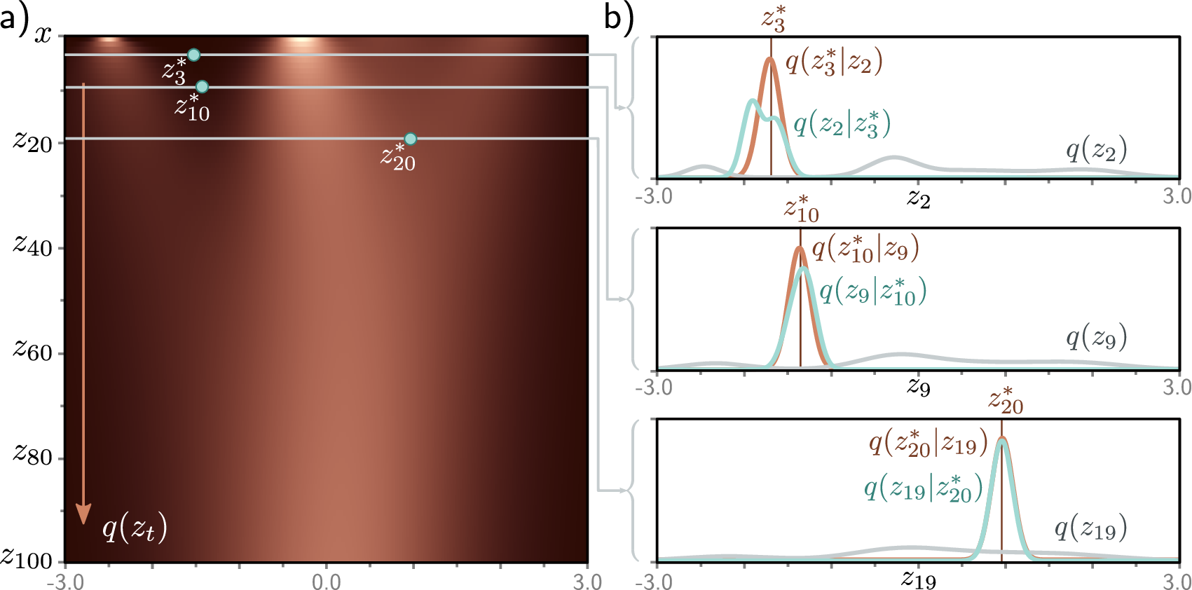
Despite their different intuitions, diffusion models and VAEs are mathematically closer than they appear. A diffusion model can be viewed as a hierarchical VAE with \(T\) latent layers \(x_1, x_2, \ldots, x_T\), where the “encoder” (forward process) is fixed rather than learned, and each layer has the same dimensionality as the data. The training objective is in fact an ELBO, decomposed into \(T\) per-timestep KL divergence terms instead of the single KL term in a standard VAE. Because both the forward posterior \(q(x_{t-1} \mid x_t, x_0)\) and the reverse model \(p_\theta(x_{t-1} \mid x_t)\) are Gaussian, each KL term reduces to an MSE between their means. Ho et al. ^[a] showed that dropping the per-timestep weighting coefficients yields \(\mathcal{L}_{\text{simple}}\), which works better in practice. For the full derivation, see Luo (2022) ¹.

Diffusion as a hierarchical VAE. A Markovian Hierarchical VAE with \(T\) latent layers. The generative (reverse) process \(p_\theta\) flows top-down along the chain; the inference (forward) process \(q\) flows bottom-up. A diffusion model is this structure with the forward process fixed to Gaussian noise addition and all latent layers sharing the data dimensionality. Source: Luo, Understanding Diffusion Models: A Unified Perspective (2022).

Per-timestep ELBO decomposition. At each step, the learned reverse distribution \(p_\theta(x_{t-1}|x_t)\) (green) is trained to match the tractable ground-truth denoising posterior \(q(x_{t-1}|x_t, x_0)\) (pink). Because both are Gaussians with matched variance, the KL divergence between them reduces to an MSE between means --- which further simplifies to the noise-prediction loss. Source: Luo, Understanding Diffusion Models: A Unified Perspective (2022).

The training procedure for a single batch is:

1. Draw a batch of clean data \(x_0\).
2. Sample random timesteps \(t \sim \mathrm{Uniform}\{1, \ldots, T\}\).
3. Sample random noise \(\epsilon \sim \mathcal{N}(0, I)\).
4. Compute noisy data \(x_t = \sqrt{\bar{\alpha}_t}\, x_0 + \sqrt{1 - \bar{\alpha}_t}\, \epsilon\).
5. Predict \(\hat{\epsilon} = \epsilon_\theta(x_t, t)\).
6. Minimize \(\lVert \epsilon - \hat{\epsilon} \rVert^2\).

def diffusion_training_loss(model: nn.Module, x0: torch.Tensor,
                            schedule: DiffusionSchedule) -> torch.Tensor:
    """Compute the simplified diffusion training loss (noise prediction MSE).

    Args:
        model: noise prediction network, takes (x_t, t) -> predicted noise
        x0: clean data batch, shape [batch, ...]
        schedule: DiffusionSchedule with precomputed quantities
    """
    batch_size = x0.size(0)

    # Step 1: sample random timesteps for each example
    t = torch.randint(0, schedule.T, (batch_size,), device=x0.device)

    # Step 2: sample Gaussian noise
    noise = torch.randn_like(x0)

    # Step 3: compute noisy version x_t
    x_t = schedule.add_noise(x0, t, noise)

    # Step 4: predict the noise
    noise_pred = model(x_t, t)

    # Step 5: MSE between true and predicted noise
    return nn.functional.mse_loss(noise_pred, noise)

This objective has a deep connection to denoising score matching². The score function \(\nabla_{x} \log p(x)\) points in the direction of increasing data density. Predicting the noise \(\epsilon\) is mathematically equivalent to estimating the score at timestep \(t\), up to a scaling factor. This connection links diffusion models to the broader framework of score-based generative modeling (Song and Ermon, 2019).

The score function as a vector field. Contour plot of a mixture of two Gaussians, overlaid with the score \(\nabla_x \log p(x)\) at each point. Arrows point toward the modes (high-density regions). The denoising network implicitly estimates this vector field at each noise level. Source: Song, Generative Modeling by Estimating Gradients of the Data Distribution (2021).

3. The Denoising Loop and Network Architecture

Generation by Iterative Denoising

Once the noise prediction network is trained, generation proceeds by simulating the reverse process. Starting from pure noise \(x_T \sim \mathcal{N}(0, I)\), we apply the learned denoising step \(T\) times:

@torch.no_grad()
def ddpm_sample(model: nn.Module, schedule: DiffusionSchedule,
                shape: tuple, device: str = "cpu") -> torch.Tensor:
    """Generate samples via DDPM reverse process.

    Args:
        model: trained noise prediction network
        schedule: DiffusionSchedule with precomputed quantities
        shape: desired output shape, e.g. (n_samples, n_residues, 3)
        device: torch device
    """
    # Start from pure Gaussian noise
    x = torch.randn(shape, device=device)

    for t in reversed(range(schedule.T)):
        t_batch = torch.full((shape[0],), t, device=device, dtype=torch.long)

        # Predict the noise component
        noise_pred = model(x, t_batch)

        # Retrieve schedule quantities for this timestep
        alpha = schedule.alphas[t]
        alpha_bar = schedule.alpha_bars[t]
        beta = schedule.betas[t]

        # Compute the predicted mean of x_{t-1}
        mean = (1.0 / torch.sqrt(alpha)) * (
            x - (beta / torch.sqrt(1.0 - alpha_bar)) * noise_pred
        )

        # Add stochastic noise for all steps except the final one
        if t > 0:
            noise = torch.randn_like(x)
            x = mean + torch.sqrt(beta) * noise
        else:
            x = mean

    return x

At each step except the last (\(t = 0\)), we inject a small amount of fresh noise. This stochasticity ensures diversity: different initial noise samples produce different outputs, and even the same initial noise can yield slightly different results due to the injected randomness during denoising.

Timestep Conditioning

The noise prediction network must know which timestep it is operating at. A heavily corrupted input (\(t\) near \(T\)) requires aggressive denoising, while a lightly corrupted input (\(t\) near 0) needs only gentle refinement. The standard approach borrows sinusoidal position embeddings from the transformer literature to encode the scalar timestep \(t\) as a high-dimensional vector:

import math

class SinusoidalTimestepEmbedding(nn.Module):
    """Encodes scalar timestep t into a d-dimensional vector.

    Uses the same sinusoidal scheme as transformer positional encodings.
    """

    def __init__(self, dim: int):
        super().__init__()
        self.dim = dim

    def forward(self, t: torch.Tensor) -> torch.Tensor:
        device = t.device
        half = self.dim // 2
        freqs = torch.exp(
            -math.log(10000.0) * torch.arange(half, device=device) / half
        )
        args = t[:, None].float() * freqs[None, :]
        return torch.cat([torch.sin(args), torch.cos(args)], dim=-1)

This embedding is then injected into the denoising network—for example, by adding it to intermediate feature maps or concatenating it with the input.

Architecture Choices for Proteins

The choice of denoising network architecture depends on the data representation.

U-Nets dominate image generation (Stable Diffusion) and medical image segmentation thanks to their multi-scale skip connections. Transformers dominate text generation thanks to their ability to capture long-range dependencies. For proteins, the choice depends on the data representation:

For spatial data (images, 3D point clouds, protein backbone coordinates), U-Net architectures with skip connections are common. The encoder half progressively reduces spatial resolution, capturing long-range context, while the decoder half restores resolution. Skip connections preserve fine-grained spatial details that would otherwise be lost during downsampling.

For sequential data (text, protein sequences), transformer architectures work well because attention allows every position to interact with every other position, capturing long-range dependencies (as discussed in Lecture 1).

For the bead-spring polymer (24 dimensions), neither U-Nets nor transformers are appropriate — the data is too small for convolutional architectures and has no sequential structure for attention. A simple MLP denoiser with a sinusoidal timestep embedding works well: the 64-dimensional timestep vector is concatenated with the 24-dimensional noisy coordinates, and three hidden layers of 256 units predict the noise. This matches the MLP architecture of the polymer VAE from Lecture 3, keeping the comparison fair (~250K parameters each).

class PolymerDenoiser(nn.Module):
    """MLP noise predictor for the bead-spring polymer."""

    def __init__(self, data_dim=24, time_dim=64, hidden_dim=256):
        super().__init__()
        self.time_embed = SinusoidalTimestepEmbedding(time_dim)
        self.net = nn.Sequential(
            nn.Linear(data_dim + time_dim, hidden_dim), nn.ReLU(),
            nn.Linear(hidden_dim, hidden_dim), nn.ReLU(),
            nn.Linear(hidden_dim, hidden_dim), nn.ReLU(),
            nn.Linear(hidden_dim, data_dim),
        )

    def forward(self, x_t, t):
        t_emb = self.time_embed(t)
        return self.net(torch.cat([x_t, t_emb], dim=-1))

4. VAEs vs. Diffusion: Choosing the Right Tool

Both VAEs and diffusion models are principled approaches to learning the distribution over proteins. They differ in architecture, training, generation speed, and sample quality. The table below summarizes the key trade-offs.

The practical upshot: VAEs win on speed (milliseconds per sample) and latent-space interpretability, making them the default for large-scale screening; diffusion wins on sample quality, making it the default for targeted design of physically plausible backbones. Latent diffusion models (Rombach et al., 2022) bridge the gap by running diffusion in a VAE’s compressed latent space, trading some quality for much faster generation.

The bead-spring polymer makes this comparison concrete. Both the VAE (Lecture 3) and DDPM (Section 6 below) are trained on the same ~10,000 preprocessed conformations with ~250K parameters each. The VAE generates 1,000 samples in ~0.01 seconds (one decoder pass); the DDPM takes ~2 seconds (200 denoising steps). The VAE’s 2D latent space reveals a smooth gradient of polymer compactness and enables gradient-based property optimization; the DDPM has no explicit latent space but produces sharper conformations. Section 6 shows these differences quantitatively.

5. Conditional Generation

Both VAEs and diffusion models can be extended to conditional generation—steering the model toward data with specific desired properties. Text-to-image models like DALL-E and Stable Diffusion generate images conditioned on text prompts; class-conditional ImageNet models generate images of specific object categories. Two general strategies have emerged for diffusion models.

Classifier guidance. Dhariwal and Nichol (2021) train a separate classifier that operates on noisy inputs. At each denoising step, the gradient of the classifier’s log-probability with respect to the noisy input is added to the predicted denoising direction, pushing the sample toward regions associated with the desired class.

Classifier-free guidance (Ho and Salimans, 2022) eliminates the need for a separate classifier. During training, the conditioning signal is randomly dropped with some probability, so the model learns both conditional and unconditional generation. At inference time, the two predictions are blended:

where \(c\) is the condition, \(\varnothing\) denotes the null condition, and \(s > 1\) amplifies the effect of conditioning. This approach is simpler and often more effective than classifier guidance. Stable Diffusion uses the guidance scale \(s\) to trade prompt adherence against visual diversity.

6. Case Study: Bead-Spring Polymer DDPM

The bead-spring polymer from Lecture 3’s VAE case study serves as a direct comparison point. Same data, same preprocessing, same parameter budget — different generative framework.

Setup

The data is identical to the VAE case study: ~10,000 polymer conformations, each a 24-dimensional vector (12 beads \(\times\) 2 coordinates), preprocessed with center-of-mass subtraction and PCA alignment. The noise schedule uses \(T = 200\) timesteps with a linear \(\beta\) schedule from \(10^{-4}\) to \(0.02\).

Denoiser Architecture

The MLP denoiser concatenates the 24-dimensional noisy coordinates with a 64-dimensional sinusoidal timestep embedding, then passes through three hidden layers of 256 units. The output is the predicted noise \(\hat{\epsilon} \in \mathbb{R}^{24}\) — the same dimensionality as the input, as required by the noise-prediction parameterization.

class PolymerDenoiser(nn.Module):
    def __init__(self, data_dim=24, time_dim=64, hidden_dim=256):
        super().__init__()
        self.time_embed = SinusoidalTimestepEmbedding(time_dim)
        self.net = nn.Sequential(
            nn.Linear(data_dim + time_dim, hidden_dim), nn.ReLU(),
            nn.Linear(hidden_dim, hidden_dim), nn.ReLU(),
            nn.Linear(hidden_dim, hidden_dim), nn.ReLU(),
            nn.Linear(hidden_dim, data_dim),
        )

    def forward(self, x_t, t):
        return self.net(torch.cat([x_t, self.time_embed(t)], dim=-1))

Training and Sampling

Training minimizes the noise-prediction MSE loss from Section 2: sample a random timestep, corrupt the polymer, predict the noise, backpropagate. The model trains for 200 epochs with Adam (learning rate \(10^{-3}\)) and batch size 256.

Generation reverses the forward process: starting from pure noise \(x_{200} \sim \mathcal{N}(0, I)\), the denoiser removes noise over 200 steps. The intermediate states form a striking visual: a random scatter of 12 points gradually coalesces into a recognizable polymer chain.

@torch.no_grad()
def sample_polymer(model, schedule, n_samples=16):
    x = torch.randn(n_samples, 24)
    for t in reversed(range(schedule.T)):
        t_batch = torch.full((n_samples,), t, dtype=torch.long)
        noise_pred = model(x, t_batch)
        alpha = schedule.alphas[t]
        alpha_bar = schedule.alpha_bars[t]
        beta = schedule.betas[t]
        mean = (1.0 / alpha.sqrt()) * (x - (beta / (1.0 - alpha_bar).sqrt()) * noise_pred)
        if t > 0:
            x = mean + beta.sqrt() * torch.randn_like(x)
        else:
            x = mean
    return x.reshape(-1, 12, 2)

Results: VAE vs. DDPM on Polymer Data

Comparing the generated conformations against training data using the radius-of-gyration distribution quantifies sample quality. Both models capture the overall shape of the \(R_g\) distribution, but they exhibit different failure modes:

• The VAE produces slightly blurred conformations — bead positions are close to correct but lack the crispness of real samples. This is the well-known “blurriness” of VAE outputs, caused by the mode-averaging effect of the MSE reconstruction loss. In exchange, the 2D latent space provides a complete map of polymer shapes, enabling smooth interpolation and gradient-based property optimization.

• The DDPM produces sharper conformations — bead positions are more precise because each denoising step makes a small, well-calibrated correction rather than a single large prediction. The cost is 200 sequential forward passes instead of one, and no explicit latent space for property optimization.

For this 24-dimensional toy system, the practical difference is small. For real proteins (thousands of dimensions), the quality gap between VAEs and diffusion models is substantial — which is why state-of-the-art protein structure generators (RFdiffusion, Chroma, FrameDiff) all use diffusion.

The full runnable code is in the nano-polymer-diffusion walkthrough, which includes side-by-side \(R_g\) histograms and timing benchmarks.

Key Takeaways

Diffusion models learn to reverse a gradual noise-corruption process. The forward process has a closed-form expression for any timestep, enabling efficient training. The reverse process is learned by predicting the noise added at each step. Generation requires many sequential denoising steps but produces state-of-the-art sample quality.

Conditional generation steers diffusion toward desired properties via classifier guidance or classifier-free guidance.

The choice between VAEs and diffusion depends on the application: VAEs for speed and interpretability, diffusion for sample quality, latent diffusion for a middle ground. The bead-spring polymer case study makes this comparison concrete on identical data: the VAE is ~200× faster and offers latent-space optimization, while the DDPM produces sharper samples.

Further Reading

• Lilian Weng, “What are Diffusion Models?” — a thorough introduction to diffusion models covering the forward process, reverse denoising, and connections to score matching.
• Yang Song, “Generative Modeling by Estimating Gradients of the Data Distribution” — score functions, noise-perturbed distributions, Langevin sampling, and SDEs for diffusion, by the score-matching pioneer.
• Calvin Luo, “Understanding Diffusion Models: A Unified Perspective” — derives diffusion from hierarchical VAEs and connects the ELBO to the score-based view via Tweedie’s formula.

References

[a] Ho, J., Jain, A., and Abbeel, P. (2020). "Denoising Diffusion Probabilistic Models." Advances in Neural Information Processing Systems (NeurIPS).