Graph Neural Networks for Protein Structures
This is Lecture 2 of the Protein & Artificial Intelligence course (Spring 2026), co-taught by Prof. Sungsoo Ahn and Prof. Homin Kim at KAIST. It assumes familiarity with transformers and attention mechanisms from Lecture 1. All code examples use PyTorch.
Introduction
A protein’s function arises from its three-dimensional fold, where residues separated by hundreds of positions in sequence come into close spatial contact. A cysteine at position 30 may form a disulfide bond with a cysteine at position 280—the spatial relationship matters more than the chain distance. Transformers process the linear sequence; graph neural networks (GNNs) process the 3D contact structure directly.
A protein structure maps naturally onto a graph: residues are nodes, spatial proximity defines edges. This representation encodes 3D structure explicitly, handles variable protein sizes without fixed-dimension constraints, and can carry rich relational information on edges—distances, angles, bond types.
This lecture develops graph neural networks from first principles. We start with the graph representation of proteins, build the message-passing framework that underlies all GNN variants, instantiate it in three concrete architectures (GCN, GAT, MPNN), and close with SE(3)-equivariant architectures that respect the rotational symmetry of 3D space.
Roadmap
| Section | Topic | Why it is needed |
|---|---|---|
| 1 | Proteins as graphs | Representing 3D structure for neural processing |
| 2 | The message-passing framework | The general GNN computation and three instantiations: GCN, GAT, MPNN |
| 3 | SE(3)-equivariant GNNs | Respecting rotational and translational symmetry of physical structures |
1. Proteins as Graphs: A Natural Representation
A protein structure maps naturally onto a graph \(G = (V, E)\). The nodes \(V\) are residues (or atoms, at finer resolution). The edges \(E\) represent spatial relationships: covalent bonds along the backbone, spatial proximity between C\(\alpha\) atoms, hydrogen bonds, salt bridges, or hydrophobic contacts.
This graph representation offers three advantages.
It encodes 3D structure directly. Instead of hoping that a sequence model will implicitly discover spatial relationships, we represent them explicitly in the graph topology.
It handles variable size naturally. Proteins range from small peptides of 50 residues to massive complexes of thousands. Graphs accommodate any number of nodes without fixed-size constraints.
It can carry rich relational information. Edges can have features describing the type and strength of interactions. You can have different edge types for backbone bonds, hydrogen bonds, and van der Waals contacts.
Here is how to convert a protein structure into a graph using PyTorch Geometric:
import torch
from torch_geometric.data import Data


def protein_to_graph(coords, sequence, k=10, threshold=10.0):
    """
    Convert a protein structure to a graph for GNN processing.

    Each residue becomes a node.  Edges connect spatially
    nearby residues based on C-alpha distances.

    Args:
        coords: (N, 3) array of C-alpha coordinates in Angstroms
        sequence: string of one-letter amino acid codes (length N)
        k: number of nearest neighbors per residue
        threshold: maximum distance (Angstroms) for an edge

    Returns:
        PyTorch Geometric Data object with node features,
        edge indices, edge attributes, and coordinates
    """
    N = len(sequence)
    coords = torch.tensor(coords, dtype=torch.float32)

    # Node features: one-hot encoding of amino acid identity (20 standard AAs)
    aa_to_idx = {aa: i for i, aa in enumerate('ACDEFGHIKLMNPQRSTVWY')}
    x = torch.zeros(N, 20)
    for i, aa in enumerate(sequence):
        if aa in aa_to_idx:
            x[i, aa_to_idx[aa]] = 1.0

    # Pairwise C-alpha distance matrix
    dist = torch.cdist(coords, coords)  # (N, N)

    # Build edges: connect each residue to its k nearest neighbors
    # within the distance threshold
    edge_index = []
    edge_attr = []

    for i in range(N):
        _, neighbors = dist[i].topk(k + 1, largest=False)
        neighbors = neighbors[1:]  # exclude self-loop

        for j in neighbors:
            if dist[i, j] < threshold:
                edge_index.append([i, j.item()])
                edge_attr.append([dist[i, j].item()])

    edge_index = torch.tensor(edge_index, dtype=torch.long).T  # (2, E)
    edge_attr = torch.tensor(edge_attr, dtype=torch.float32)    # (E, 1)

    return Data(x=x, edge_index=edge_index, edge_attr=edge_attr, pos=coords)
2. The Message-Passing Framework
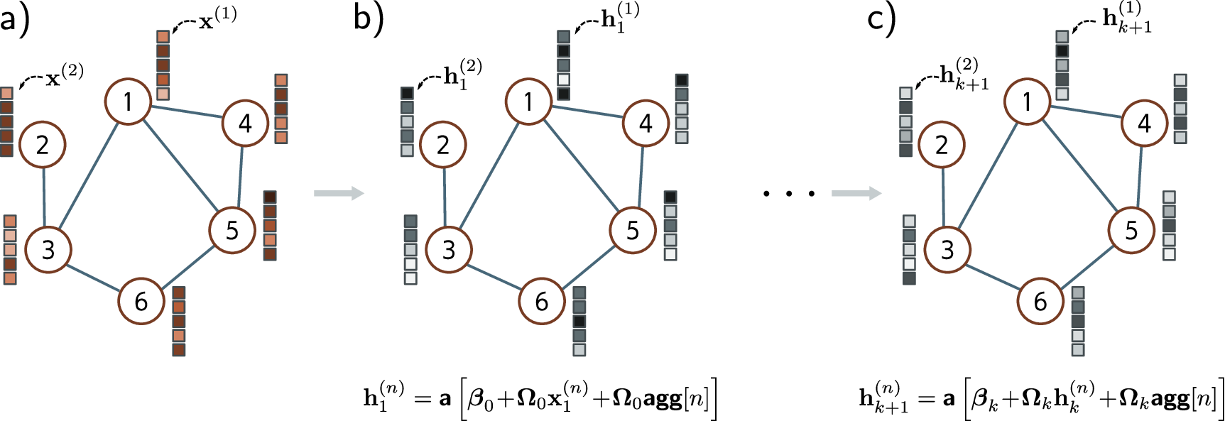
Message passing generalizes beyond proteins. In social networks, a user’s interests can be predicted from their friends’ profiles. In citation networks, a paper’s topic is inferred from the papers it cites and the papers that cite it. All graph neural networks share a common computational pattern called message passing. The intuition is straightforward: each node gathers information from its neighbors, combines it, and updates its own representation.
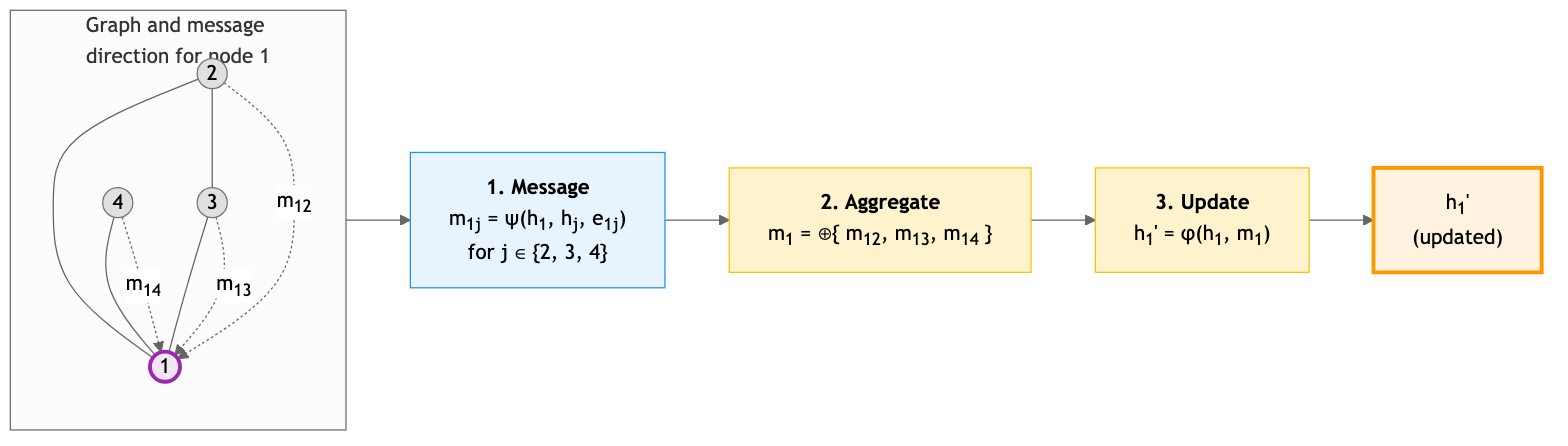
Think of yourself as a residue in a folded protein. You want to refine your representation based on your structural neighborhood. You ask each neighbor to send you a message about its current state. You aggregate all incoming messages, combine them with your own state, and produce an updated representation.
Formally, a single message-passing layer computes:
\[h_i^{(\ell+1)} = \phi\!\left(h_i^{(\ell)},\; \bigoplus_{j \in \mathcal{N}(i)} \psi\!\left(h_i^{(\ell)},\, h_j^{(\ell)},\, e_{ij}\right)\right)\]The symbols in this equation deserve careful definition:
- \(h_i^{(\ell)} \in \mathbb{R}^{d}\) is the representation (feature vector) of node \(i\) at layer \(\ell\).
- \(\mathcal{N}(i)\) is the set of neighbors of node \(i\) in the graph.
- \(e_{ij} \in \mathbb{R}^{d_e}\) is the edge feature between nodes \(i\) and \(j\) (e.g., inter-residue distance).
- \(\psi\) is the message function: given the states of two connected nodes and their edge feature, it computes the message to send.
- \(\bigoplus\) is the aggregation function: it combines messages from all neighbors into a single vector. Common choices are sum, mean, and max.
- \(\phi\) is the update function: it combines the node’s current state with the aggregated messages to produce the updated state.
Different GNN architectures correspond to different choices of \(\psi\), \(\bigoplus\), and \(\phi\). The three most important variants are described below.
Graph Convolutional Networks (GCN)
The GCN (Kipf and Welling, 2017) is the simplest GNN. Each node averages its own features and its neighbors’ features, applies a shared linear transformation \(W^{(\ell)} \in \mathbb{R}^{d \times d'}\), and passes the result through a nonlinearity:
\[h_i^{(\ell+1)} = \sigma\!\left(\frac{1}{|\mathcal{N}(i)|}\sum_{j \in \mathcal{N}(i)} W^{(\ell)}\, h_j^{(\ell)}\right)\]where \(\mathcal{N}(i)\) includes node \(i\) itself (self-loop). The limitation: GCN treats all neighbors equally—it cannot learn that some matter more than others.
Graph Attention Networks (GAT)
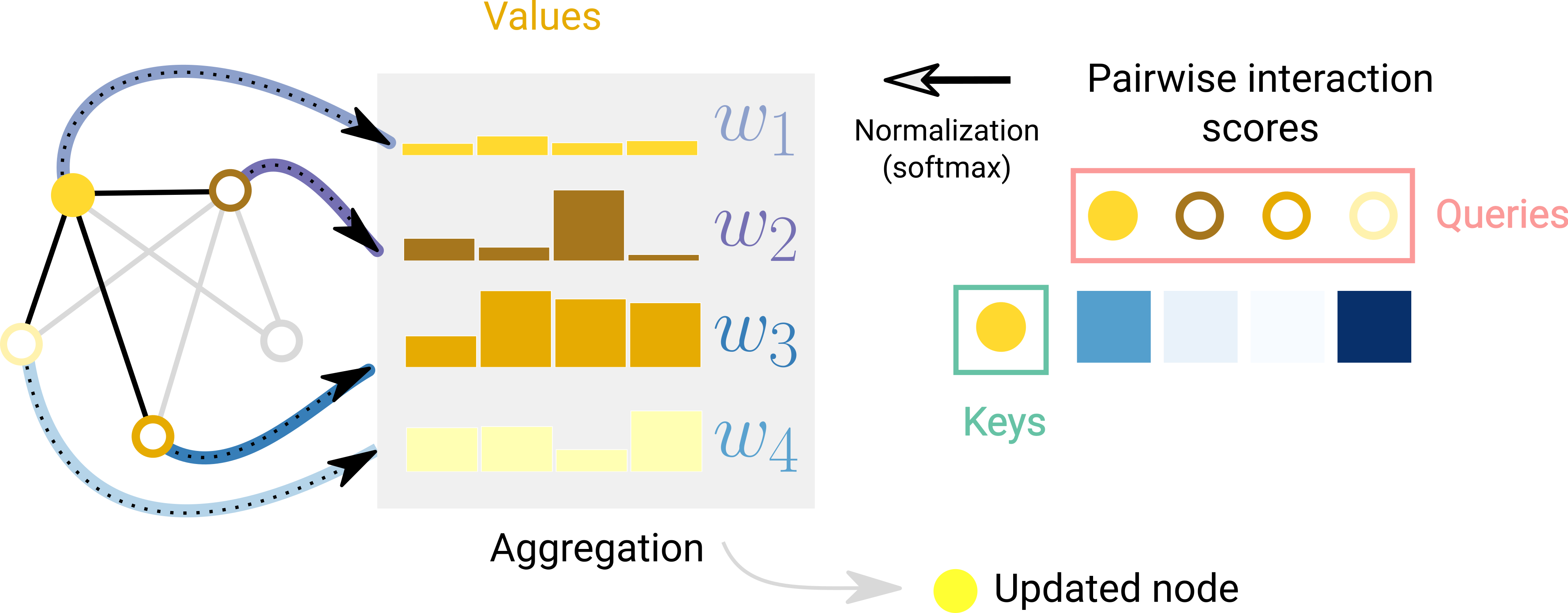
The GAT (Veličković et al., 2018) addresses this limitation by computing learned attention coefficients \(\alpha_{ij}\) between each node and its neighbors, then taking a weighted sum instead of a uniform average:
\[h_i^{(\ell+1)} = \sigma\!\left(\sum_{j \in \mathcal{N}(i)} \alpha_{ij}\, W^{(\ell)} h_j^{(\ell)}\right)\]The coefficients \(\alpha_{ij}\) are computed by a small neural network (a learnable vector \(\mathbf{a} \in \mathbb{R}^{2d'}\) applied to the concatenation of transformed node features), then normalized with softmax over the neighborhood. Like the transformer, GAT supports multi-head attention—each head learns different interaction patterns.
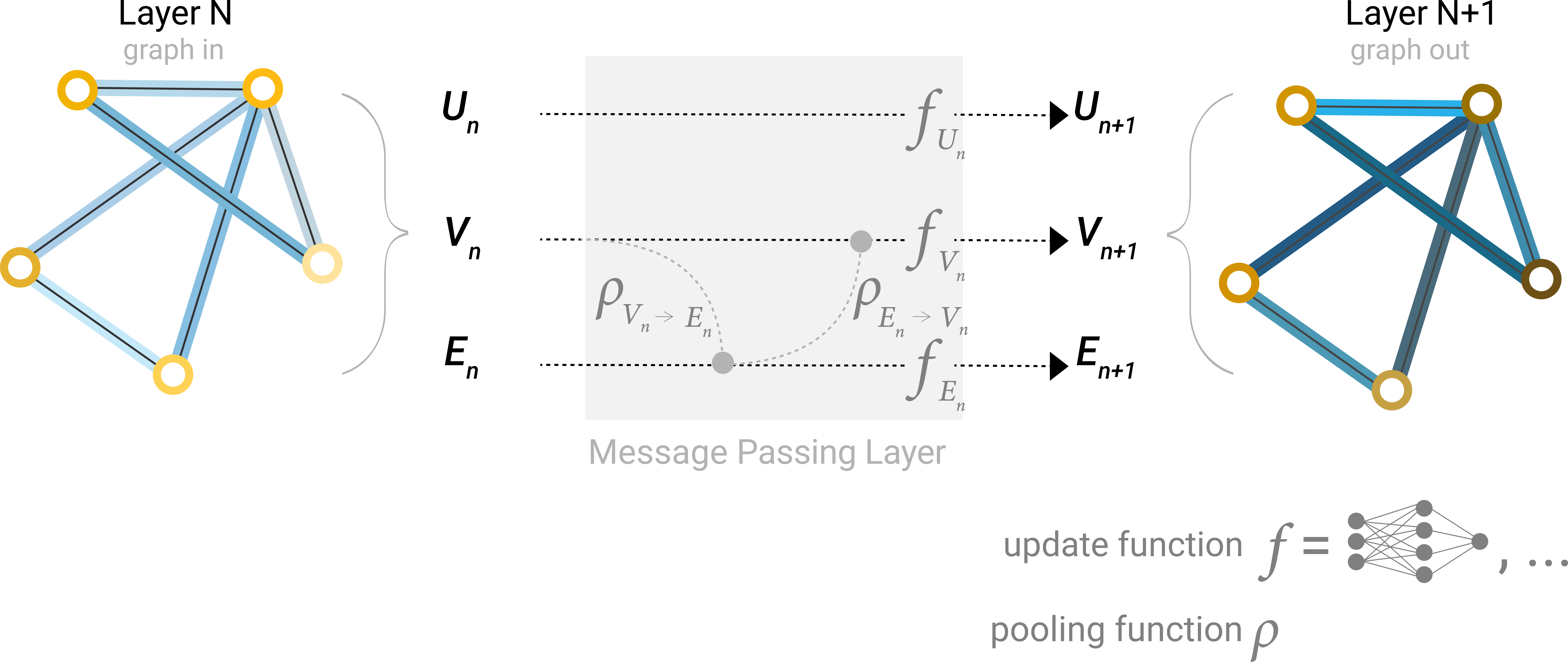
Message Passing Neural Networks (MPNN)
The MPNN framework (Gilmer et al., 2017) provides maximum flexibility by replacing the fixed message rules of GCN and the specific attention mechanism of GAT with arbitrary learned networks:
\[m_{ij} = M_\theta\!\left(h_i^{(\ell)},\, h_j^{(\ell)},\, e_{ij}\right), \qquad h_i^{(\ell+1)} = U_\theta\!\left(h_i^{(\ell)},\, \sum_{j \in \mathcal{N}(i)} m_{ij}\right)\]Here \(M_\theta\) and \(U_\theta\) are learned MLPs. The key advantage for proteins is that \(M_\theta\) can incorporate rich edge features \(e_{ij}\)—inter-residue distances, backbone angles, sequence separation—which GCN and GAT cannot naturally handle. This makes MPNN the architecture of choice for structure-based protein design, as exemplified by ProteinMPNN (Dauparas et al., 2022).
3. SE(3)-Equivariant GNNs: Respecting Physical Symmetry
When we work with 3D protein structures, there is a fundamental physical principle we should respect: the laws of physics do not depend on how we orient the coordinate system. A protein’s energy, its stability, and its function are the same whether we describe its coordinates in one frame or another.
This symmetry principle is formalized by the group SE(3)—the group of all rigid-body transformations in three dimensions, comprising rotations and translations1.
An SE(3)-equivariant model produces outputs that transform consistently under coordinate changes. Let \(R \in \mathbb{R}^{3 \times 3}\) be a rotation matrix and \(t \in \mathbb{R}^3\) a translation vector. If we apply this rigid-body transformation to every atom coordinate \(\mathbf{r}_i \mapsto R\mathbf{r}_i + t\), then:
- Invariant outputs (scalars such as energy or binding affinity) should not change at all:
- Equivariant outputs (vectors such as forces or coordinate updates) should rotate along with the input:
Standard GNNs that operate on raw coordinates satisfy neither property. If you rotate the input coordinates, the outputs change unpredictably. The model must therefore waste capacity learning the same function for every possible orientation, and it may generalize poorly to orientations not seen during training.
SE(3)-equivariant GNNs solve this by designing the message-passing operations to respect 3D symmetry. The key strategies include:
- Operating on invariant quantities such as pairwise distances \(\lvert\mathbf{r}_i - \mathbf{r}_j\rvert\) (where \(\mathbf{r}_i \in \mathbb{R}^3\) is the coordinate of node \(i\)) and angles, which do not change under rotation.
- Processing equivariant quantities such as direction vectors \(\mathbf{r}_i - \mathbf{r}_j\) using operations that commute with rotation.
- Decomposing features by transformation behavior. Some architectures use tools from group representation theory to decompose features into components that transform predictably under rotation — scalars that do not change, vectors that rotate, and higher-order objects that transform according to specific rules.
Prominent examples of SE(3)-equivariant architectures include:
- Tensor Field Networks (TFN) and SE(3)-Transformers, which use more advanced mathematical machinery from group representation theory to achieve exact equivariance for features of arbitrary order.
- E(n) Equivariant Graph Neural Networks (EGNN), which achieve equivariance through a simpler mechanism of updating coordinates using displacement vectors scaled by learned scalar weights.
- Invariant Point Attention (IPA), the architecture used in AlphaFold’s structure module, which applies attention in local residue frames to achieve equivariance.
The core insight is practical: by building the right symmetries into our models, we get better generalization with less data. The model does not need to learn that a rotated protein has the same energy as the original—this is guaranteed by construction.
Key Takeaways
-
Graph neural networks represent proteins as graphs, naturally encoding 3D structural relationships through the message-passing framework.
-
GCN, GAT, and MPNN are three instantiations of the message-passing framework with increasing flexibility: GCN uses fixed neighbor averaging, GAT learns attention weights over neighbors, and MPNN uses fully learnable message and update functions.
-
SE(3)-equivariant GNNs respect the rotational and translational symmetry of physical space, providing better generalization on 3D structure tasks.
-
Transformers and equivariant GNNs are complementary: transformers capture long-range sequence dependencies while equivariant GNNs respect the symmetries of 3D structure. Their combination powers models like AlphaFold.
Further Reading
- Sanchez-Lengeling et al., “A Gentle Introduction to Graph Neural Networks” — interactive introduction to GNNs covering graph representations and message passing.
- Daigavane et al., “Understanding Convolutions on Graphs” — companion piece on spectral and spatial graph convolutions.
- Fabian Fuchs, “SE(3)-Transformers” — equivariant self-attention on 3D point clouds and roto-translation equivariance.
- Andrew White, “Equivariant Neural Networks” — textbook chapter deriving E(3)-equivariant GNNs from group theory, with code examples.
-
SE(3) stands for “Special Euclidean group in 3 dimensions.” It is the set of all transformations of the form \(x \mapsto Rx + t\), where \(R \in \mathbb{R}^{3 \times 3}\) is a rotation matrix (\(R^T R = I\), \(\det R = 1\)) and \(t \in \mathbb{R}^{3}\) is a translation vector. ↩