ProteinMPNN: Architecture and Training
This is Lecture 12 of the Protein & Artificial Intelligence course (Spring 2026), co-taught by Prof. Sungsoo Ahn and Prof. Homin Kim at KAIST Graduate School of AI. This is the architecture companion to Lecture 11 (Inverse Folding and the Design Pipeline). Assumes familiarity with graph neural networks (Lecture 2) and the inverse folding problem (Lecture 11). All code examples use PyTorch.
Introduction
Lecture 11 framed the inverse folding problem and the design pipeline. This lecture opens the hood: how ProteinMPNN represents protein structure as a graph, encodes geometric relationships between residues, and generates sequences one amino acid at a time.
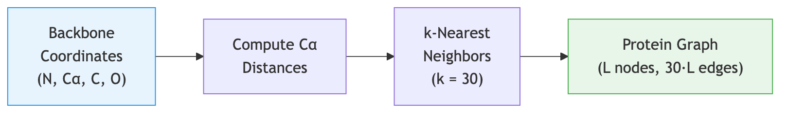
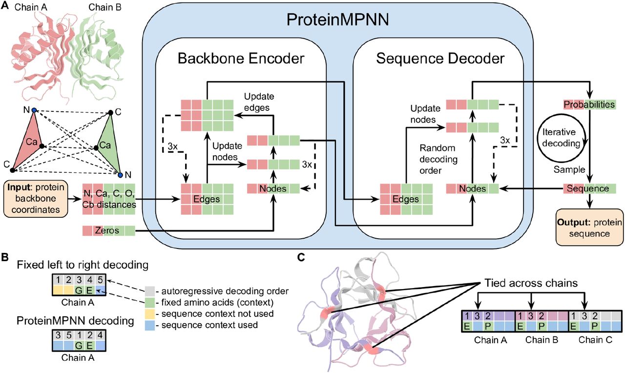
The architecture has three stages. First, backbone coordinates are converted into a k-nearest neighbor graph where each residue connects to its spatially closest neighbors. Second, a message-passing encoder propagates structural information across the graph, building context-aware representations for every residue. Third, an autoregressive decoder generates amino acids one position at a time, conditioned on the structure encoding and all previously decoded positions. The decoding order is randomized during training, so the model learns to predict any position given any subset of context.
Roadmap
| Section | Topic | Why It Is Needed |
|---|---|---|
| 1 | Graph Construction | Translates raw backbone coordinates into a data structure that neural networks can process |
| 2 | Edge Features | Provides a rich geometric vocabulary beyond simple distances |
| 3 | The Structure Encoder | Propagates local geometric information across the protein through message passing |
| 4 | Autoregressive Decoding | Generates amino acids one at a time, capturing inter-residue dependencies |
| 5 | Training | Describes the loss function, random-order training, and data augmentation |
| 6 | Advanced Features | Handles practical constraints: fixed positions, symmetry, and tied sequences |
1. Graph Construction: Proteins as k-Nearest Neighbor Graphs
The first step in ProteinMPNN’s pipeline is converting a protein backbone into a graph. This is where the geometric nature of the problem gets translated into a form that a neural network can process.
Why Graphs?
Proteins have an obvious graph-like quality. Each residue is a discrete unit (a natural node), and the spatial relationships between residues define natural edges. Unlike images, which live on regular grids, protein structures are irregular: residues that are far apart in the amino acid sequence may be close together in three-dimensional space because the chain folds back on itself. Graph neural networks handle this irregularity natively.
Building the k-NN Graph
For each residue, ProteinMPNN finds its \(k\) nearest neighbors based on the Euclidean distance between their alpha-carbon (\(\text{C}_\alpha\)) atoms. A typical choice is \(k = 30\), meaning each residue connects to its 30 closest spatial neighbors.
Why \(\text{C}_\alpha\) distances? The alpha-carbon sits at the geometric center of each amino acid’s backbone, making it a stable reference point for the overall residue position. While more elaborate distance measures are possible (e.g., using multiple backbone atoms), \(\text{C}_\alpha\) distances are effective and computationally cheap.
import torch
import torch.nn as nn

def build_knn_graph(ca_coords, k=30, exclude_self=True):
    """
    Build a k-nearest neighbor graph from alpha-carbon coordinates.

    Args:
        ca_coords: [L, 3] tensor of C-alpha positions for L residues.
        k: Number of neighbors per residue.
        exclude_self: If True, a residue cannot be its own neighbor.

    Returns:
        edge_index: [2, E] tensor where E = L * k. Row 0 is source, row 1 is destination.
        edge_dist:  [E] tensor of Euclidean distances for each edge.
    """
    L = ca_coords.shape[0]

    # Pairwise distance matrix: dist[i, j] = ||CA_i - CA_j||
    diff = ca_coords.unsqueeze(0) - ca_coords.unsqueeze(1)  # [L, L, 3]
    dist = diff.norm(dim=-1)  # [L, L]

    if exclude_self:
        dist.fill_diagonal_(float('inf'))  # prevent self-loops

    # For each residue, select the k nearest neighbors
    _, neighbors = dist.topk(k, dim=-1, largest=False)  # [L, k]

    # Flatten into edge list
    src = torch.arange(L).unsqueeze(-1).expand(-1, k).reshape(-1)
    dst = neighbors.reshape(-1)
    edge_index = torch.stack([src, dst])  # [2, L*k]

    edge_dist = dist[src, dst]  # [L*k]

    return edge_index, edge_dist
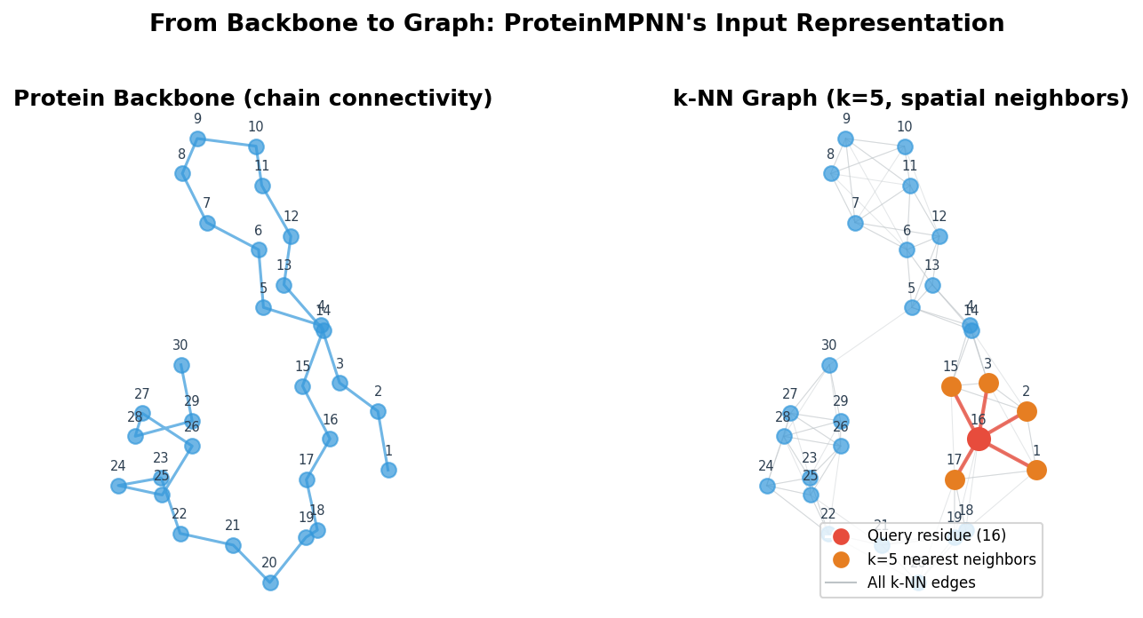
This construction captures something important about tertiary structure. Two residues that are 50 positions apart in the sequence might be less than 5 angstroms apart in space because the chain has folded back on itself. By using spatial rather than sequence neighborhoods, the graph encodes exactly these long-range contacts that define the protein’s three-dimensional shape.
2. Edge Features: Encoding Spatial Relationships
A single distance number between two residues is not enough to describe their geometric relationship. Two residue pairs might both be 8 angstroms apart, yet one pair could be in a parallel beta-sheet (side by side, pointing the same direction) while the other is in an antiparallel arrangement (side by side, pointing opposite directions). ProteinMPNN uses a rich set of edge features to capture these distinctions.
Radial Basis Function (RBF) Distance Encoding
Rather than feeding the raw distance to the network, ProteinMPNN passes it through a set of Gaussian basis functions. Given a distance \(d\), the RBF encoding produces a vector:
\[\text{RBF}(d) = \left[\exp\left(-\gamma (d - \mu_1)^2\right),\; \exp\left(-\gamma (d - \mu_2)^2\right),\; \dots,\; \exp\left(-\gamma (d - \mu_K)^2\right)\right]\]where \(\mu_1, \mu_2, \dots, \mu_K\) are evenly spaced centers between 0 and a maximum distance (e.g., 20 angstroms), and \(\gamma\) controls the width of each Gaussian. This encoding is smooth and differentiable, and it allows the network to treat different distance ranges with separate learned weights.
def rbf_encode(distances, num_rbf=16, max_dist=20.0):
    """
    Encode distances using radial basis functions.

    Args:
        distances: [E] tensor of pairwise distances.
        num_rbf: Number of Gaussian basis functions.
        max_dist: Maximum distance covered by the basis centers.

    Returns:
        rbf: [E, num_rbf] tensor of RBF-encoded distances.
    """
    centers = torch.linspace(0, max_dist, num_rbf, device=distances.device)
    gamma = num_rbf / max_dist
    return torch.exp(-gamma * (distances.unsqueeze(-1) - centers) ** 2)
Local Coordinate Frames
Each residue has a natural local coordinate system defined by its three backbone atoms: N, \(\text{C}_\alpha\), and C. These three atoms define a plane, and from that plane we can construct an orthonormal frame1:
- The x-axis points from \(\text{C}_\alpha\) toward C.
- The z-axis is perpendicular to the N-\(\text{C}_\alpha\)-C plane (computed via a cross product).
- The y-axis completes the right-handed coordinate system.
def compute_local_frame(N, CA, C):
    """
    Compute a local coordinate frame from backbone atoms N, CA, C.

    Args:
        N:  [..., 3] nitrogen positions.
        CA: [..., 3] alpha-carbon positions.
        C:  [..., 3] carbonyl carbon positions.

    Returns:
        R: [..., 3, 3] rotation matrix (columns are x, y, z axes).
        t: [..., 3] translation (the CA position).
    """
    # x-axis: CA -> C direction
    x = C - CA
    x = x / (x.norm(dim=-1, keepdim=True) + 1e-8)

    # z-axis: perpendicular to the N-CA-C plane
    v = N - CA
    z = torch.cross(x, v, dim=-1)
    z = z / (z.norm(dim=-1, keepdim=True) + 1e-8)

    # y-axis: completes the right-handed frame
    y = torch.cross(z, x, dim=-1)

    R = torch.stack([x, y, z], dim=-1)  # [..., 3, 3]
    return R, CA
Direction and Orientation Features
Using the local frames, ProteinMPNN computes several additional edge features for each pair of connected residues \(i\) and \(j\):
- Direction vectors. The vector from residue \(i\) to residue \(j\), expressed in residue \(i\)’s local frame (and vice versa). This tells the network whether neighbor \(j\) is “in front of,” “behind,” “above,” or “below” residue \(i\).
- Orientation features. Dot products between the axes of frames \(i\) and \(j\). These capture whether two residues are pointing in the same direction, perpendicular to each other, or antiparallel.
- Sequence separation. The difference \(\lvert j - i \rvert\) in sequence position. This distinguishes local contacts (expected from chain connectivity) from long-range contacts (which carry more structural information).
Together, these features give the network a rich geometric vocabulary. Rather than learning from scratch what an “alpha helix” or “beta sheet” looks like, the network receives information that already encodes many of the relevant structural motifs.
3. The Structure Encoder: Message Passing
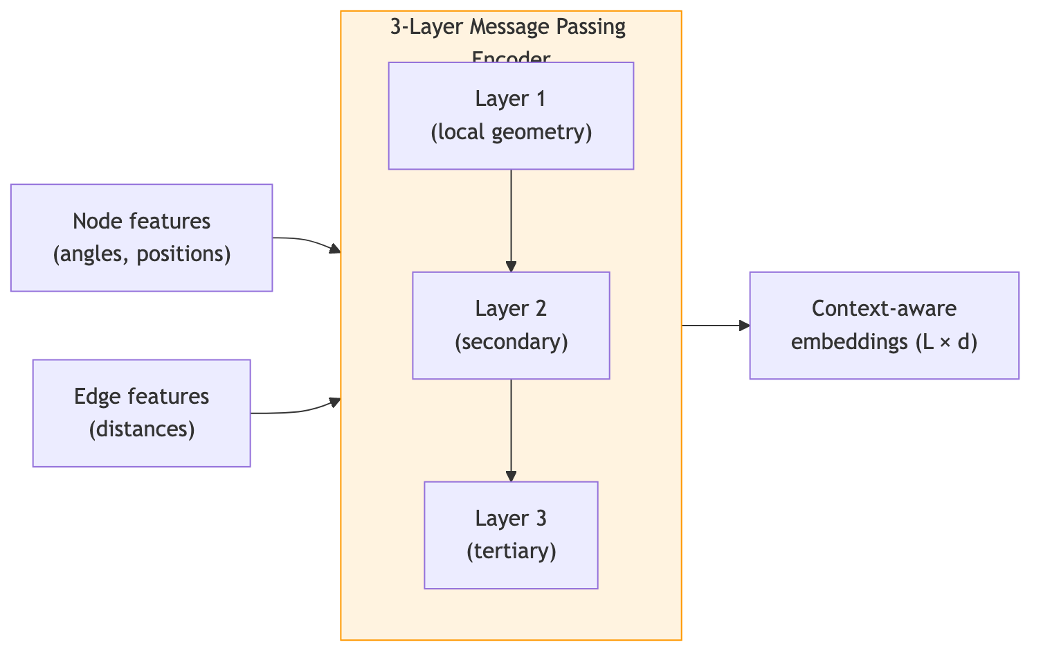
With the graph constructed and edge features computed, the structure encoder integrates information across the protein. Its mechanism is message passing—a paradigm from graph neural networks where each node iteratively gathers information from its neighbors2.
How Message Passing Works
Each node (residue) in the graph maintains a feature vector \(\mathbf{h}_i\). At each layer of the encoder, three operations occur:
-
Message computation. For each edge \((i, j)\), a message \(\mathbf{m}_{j \to i}\) is computed from the features of both endpoints and the edge:
\[\mathbf{m}_{j \to i} = f_{\text{msg}}\!\left(\mathbf{h}_i,\; \mathbf{h}_j,\; \mathbf{e}_{ij}\right)\]where \(f_{\text{msg}}\) is a learned MLP and \(\mathbf{e}_{ij}\) is the edge feature vector.
-
Aggregation. Each residue sums the messages from all its neighbors:
\[\mathbf{a}_i = \sum_{j \in \mathcal{N}(i)} \mathbf{m}_{j \to i}\]The sum is permutation-invariant—the order of neighbors does not matter.
-
Update. Each residue updates its feature vector using its old state and the aggregated messages:
\[\mathbf{h}_i^{(\ell+1)} = f_{\text{upd}}\!\left(\mathbf{h}_i^{(\ell)},\; \mathbf{a}_i\right)\]with residual connections and layer normalization for stable training.
After \(\ell\) layers, each residue’s representation encodes information from residues up to \(\ell\) hops away in the graph. With \(k = 30\) neighbors and 3 layers (the typical depth in ProteinMPNN), the receptive field covers a substantial portion of the protein’s local structural environment.
class MPNNLayer(nn.Module):
    """Single message-passing layer for the structure encoder."""

    def __init__(self, hidden_dim, dropout=0.1):
        super().__init__()
        self.hidden_dim = hidden_dim

        # Message function: takes [h_i, h_j, e_ij] and produces a message vector
        self.message_mlp = nn.Sequential(
            nn.Linear(hidden_dim * 3, hidden_dim),
            nn.ReLU(),
            nn.Linear(hidden_dim, hidden_dim),
            nn.Dropout(dropout),
        )

        # Update function: takes [h_i, aggregated_messages] and produces updated h_i
        self.update_mlp = nn.Sequential(
            nn.Linear(hidden_dim * 2, hidden_dim),
            nn.ReLU(),
            nn.Linear(hidden_dim, hidden_dim),
            nn.Dropout(dropout),
        )

        self.norm1 = nn.LayerNorm(hidden_dim)
        self.norm2 = nn.LayerNorm(hidden_dim)

    def forward(self, h, e, edge_index):
        """
        Args:
            h: [L, hidden_dim] node features for L residues.
            e: [E, hidden_dim] edge features for E edges.
            edge_index: [2, E] source and destination indices.

        Returns:
            h_new: [L, hidden_dim] updated node features.
        """
        src, dst = edge_index
        L = h.shape[0]

        # Step 1: Compute messages m_{src -> dst}
        msg_input = torch.cat([h[src], h[dst], e], dim=-1)
        messages = self.message_mlp(msg_input)  # [E, hidden_dim]

        # Step 2: Aggregate messages at each destination node
        aggregated = torch.zeros(L, self.hidden_dim, device=h.device)
        aggregated.scatter_add_(
            0, dst.unsqueeze(-1).expand(-1, self.hidden_dim), messages
        )

        # Step 3: Update node features with residual connection
        h_res = self.norm1(h + aggregated)
        h_new = h_res + self.update_mlp(torch.cat([h_res, aggregated], dim=-1))
        h_new = self.norm2(h_new)

        return h_new
After three such layers, each residue’s representation captures not just its own local geometry but the shape of nearby secondary structure elements, the positioning of core versus surface, and the presence of cavities or channels. This contextual encoding is the foundation on which the decoder builds.
4. Autoregressive Decoding: One Amino Acid at a Time

Given the encoded structure, ProteinMPNN generates a sequence autoregressively: one amino acid at a time, where each prediction depends on all previous predictions.
The Autoregressive Factorization
Let \(\mathbf{s} = (s_1, s_2, \dots, s_L)\) denote the sequence and \(\mathcal{X}\) the backbone structure. The autoregressive approach factorizes the joint probability as:
\[P(\mathbf{s} \mid \mathcal{X}) = \prod_{i=1}^{L} P\!\left(s_{\pi(i)} \mid s_{\pi(1)}, \dots, s_{\pi(i-1)},\; \mathcal{X}\right)\]where \(\pi\) is a permutation that defines the decoding order (discussed below). Each factor represents the probability of the amino acid at position \(\pi(i)\), conditioned on the backbone structure and all amino acids decoded before it.
This factorization has three advantages over predicting all positions simultaneously3:
- Captures dependencies. If you place a positively charged lysine at one position, a nearby position might prefer a negatively charged glutamate for favorable electrostatic interaction. Autoregressive generation models these pairwise preferences naturally.
- Exact likelihoods. The log-probability \(\log P(\mathbf{s} \mid \mathcal{X})\) can be computed exactly by summing the log-probabilities at each step. This is useful for ranking and filtering designs.
- Flexible constraints. Certain positions can be fixed, sampling randomness can be adjusted, or other constraints can be applied during generation without retraining.
Random Decoding Order
In language models, tokens are generated left to right because that matches how we read. For proteins, there is no privileged direction—the N-terminus is not inherently more important than the C-terminus.
ProteinMPNN uses a random decoding order during training. Each training example uses a different random permutation \(\pi\). This has three important consequences:
- Order-agnostic learning. The model learns to predict any position given any subset of other positions, making it flexible at inference time.
- Bidirectional context. When decoding position \(i\), the model may have already decoded positions both before and after \(i\) in the sequence. This provides richer context than strict left-to-right generation.
- Reduced bias. N-to-C decoding would create an asymmetry where early positions are predicted with less context than late positions. Random order averages out this bias over many training iterations.
The decoding order is enforced through a causal mask that prevents each position from attending to positions that have not yet been decoded.
def create_decoding_mask(decoding_order):
    """
    Create a causal attention mask for an arbitrary decoding order.

    Args:
        decoding_order: [L] tensor. decoding_order[step] = position decoded at that step.

    Returns:
        mask: [L, L] boolean tensor.
              mask[i, j] = True means position i CANNOT attend to position j.
    """
    L = decoding_order.shape[0]

    # order_idx[pos] = the step at which position pos is decoded
    order_idx = torch.zeros(L, dtype=torch.long, device=decoding_order.device)
    order_idx[decoding_order] = torch.arange(L, device=decoding_order.device)

    # Position i can attend to position j only if j was decoded before i
    # i.e., order_idx[j] < order_idx[i]
    mask = order_idx.unsqueeze(0) >= order_idx.unsqueeze(1)  # [L, L]

    return mask
Sampling Strategies
Once the model is trained, the diversity of generated sequences is controlled through sampling strategies that adjust the trade-off between confidence and exploration.
Temperature sampling. Let \(z_i\) denote the logit (raw network output) for amino acid \(i\). The sampling probability is:
\[P(s = i) = \frac{\exp(z_i / T)}{\sum_{j=1}^{20} \exp(z_j / T)}\]where \(T\) is the temperature. When \(T < 1\), the distribution sharpens toward the most likely amino acid. When \(T > 1\), the distribution flattens, giving rare amino acids a higher chance. In practice, temperatures of 0.1–0.3 produce conservative, high-confidence designs; temperatures near 1.0 explore more diverse alternatives.
Top-\(k\) sampling. Only the \(k\) amino acids with the highest logits are considered; all other probabilities are set to zero. This prevents sampling extremely unlikely amino acids while preserving diversity among the top choices.
Top-\(p\) (nucleus) sampling. The smallest set of amino acids whose cumulative probability exceeds a threshold \(p\) is selected. If one amino acid dominates (e.g., 95% probability), only that amino acid is considered. If the distribution is flat, many amino acids remain in the candidate set. This adaptive behavior makes top-\(p\) sampling more robust than a fixed top-\(k\).
def sample_sequence(model, structure_encoding, temperature=0.1,
                    top_k=None, decoding_order=None):
    """
    Sample a complete amino acid sequence from ProteinMPNN.

    Args:
        model: Trained ProteinMPNN model.
        structure_encoding: [L, hidden_dim] encoded backbone features.
        temperature: Sampling temperature (lower = more deterministic).
        top_k: If set, only consider the top-k most likely amino acids.
        decoding_order: [L] permutation. Random if None.

    Returns:
        sequence:  [L] tensor of sampled amino acid indices (0-19).
        log_probs: [L] tensor of log-probabilities at each position.
    """
    L = structure_encoding.shape[0]
    device = structure_encoding.device
    NUM_AMINO_ACIDS = 20
    MASK_TOKEN = 21  # special token for "not yet decoded"

    if decoding_order is None:
        decoding_order = torch.randperm(L, device=device)

    sequence = torch.full((L,), MASK_TOKEN, device=device, dtype=torch.long)
    log_probs = torch.zeros(L, device=device)

    for step in range(L):
        pos = decoding_order[step].item()

        # Get logits for this position, conditioned on structure + decoded residues
        mask = create_decoding_mask(decoding_order[:step + 1])
        logits = model.decoder(
            structure_encoding.unsqueeze(0),
            sequence.unsqueeze(0),
            decoding_order,
            mask,
        )
        logits = logits[0, pos, :NUM_AMINO_ACIDS]  # [20]

        # Apply temperature
        logits = logits / temperature

        # Optional top-k filtering
        if top_k is not None:
            topk_vals, topk_idx = logits.topk(top_k)
            logits = torch.full_like(logits, float('-inf'))
            logits[topk_idx] = topk_vals

        # Sample from the distribution
        probs = torch.softmax(logits, dim=-1)
        aa = torch.multinomial(probs, num_samples=1).item()

        sequence[pos] = aa
        log_probs[pos] = torch.log(probs[aa])

    return sequence, log_probs
5. Training: Learning from Nature’s Designs
Training ProteinMPNN is conceptually straightforward: show the model millions of protein structures paired with their natural sequences, and train it to predict the sequence given the structure. Several details make this work well in practice.
Loss Function
The training objective is the negative log-likelihood of the true sequence under the model’s autoregressive distribution:
\[\mathcal{L} = -\sum_{i=1}^{L} \log P\!\left(s_i^{\text{true}} \mid s_{<i}^{\text{true}},\; \mathcal{X}\right)\]This is equivalent to cross-entropy loss between the predicted amino acid probabilities and the true amino acids at each position. During training, the model uses teacher forcing: it conditions on the true previous amino acids rather than its own predictions, which makes training efficient and fully parallelizable across positions.
Random Order Training
At each training iteration, a fresh random permutation \(\pi\) is sampled for each protein in the batch. This ensures the model cannot rely on a fixed decoding direction and must learn to predict any position given any subset of context positions.
def train_step(model, batch, optimizer, device):
    """
    One training step for ProteinMPNN.

    Args:
        model: The ProteinMPNN model.
        batch: Dictionary with 'coords' (backbone atoms) and 'sequence' (true AAs).
        optimizer: PyTorch optimizer.
        device: Computation device.

    Returns:
        loss: Scalar training loss for this batch.
    """
    model.train()

    coords = {k: v.to(device) for k, v in batch['coords'].items()}
    sequence = batch['sequence'].to(device)  # [L] true amino acid indices
    L = sequence.shape[0]

    # Sample a fresh random decoding order for this example
    decoding_order = torch.randperm(L, device=device)

    # Forward pass: predict amino acid logits at each position
    logits = model(coords, sequence, decoding_order)  # [L, 20]

    # Cross-entropy loss against the true sequence
    loss = nn.functional.cross_entropy(
        logits.view(-1, 20),
        sequence.view(-1),
        reduction='mean',
    )

    optimizer.zero_grad()
    loss.backward()
    optimizer.step()

    return loss.item()
Data Augmentation
Real experimental structures contain measurement errors, conformational flexibility, and occasional mistakes. ProteinMPNN uses two forms of data augmentation to build robustness:
Coordinate noise. Small Gaussian noise (standard deviation \(\sim\) 0.1 angstroms) is added to backbone atom positions. This simulates the uncertainty in experimental coordinates and prevents the model from relying on overly precise geometric details that would not be present in computationally designed backbones.
Random cropping. Training on random contiguous segments of proteins helps the model generalize across protein sizes and prevents memorization of specific proteins.
def augment_structure(coords, noise_prob=0.1, noise_std=0.1):
    """
    Add Gaussian noise to backbone coordinates with some probability.

    Args:
        coords: Dictionary mapping atom names ('N', 'CA', 'C', 'O') to [L, 3] tensors.
        noise_prob: Probability of applying noise.
        noise_std: Standard deviation of Gaussian noise in angstroms.

    Returns:
        coords: Augmented coordinates (modified in-place).
    """
    if torch.rand(1).item() < noise_prob:
        for atom_name in coords:
            coords[atom_name] = coords[atom_name] + torch.randn_like(coords[atom_name]) * noise_std
    return coords
Training Data
The original ProteinMPNN was trained on experimentally determined protein structures from the Protein Data Bank (PDB). The training set includes tens of thousands of protein chains spanning diverse folds, sizes, and functions. Structures are filtered by resolution (typically \(\leq\) 3.5 angstroms) and redundancy (removing near-identical chains) to ensure a high-quality, non-redundant training set.
6. Advanced Features: Constraints and Symmetry
Real protein design problems come with constraints. You may need to keep certain catalytic residues unchanged, or you may be designing a symmetric oligomer where all chains must share the same sequence. ProteinMPNN handles both cases cleanly.
Fixed Position Conditioning
Suppose you have a validated binding interface and want to redesign only the rest of the protein for improved stability. The approach is straightforward: set the binding-site residues to their known amino acids and exclude them from the decoding order. The decoder then conditions on these fixed positions when generating the remaining sequence.
def design_with_fixed_positions(model, coords, fixed_positions, fixed_aas):
    """
    Design a sequence with certain positions held fixed.

    Args:
        model: Trained ProteinMPNN.
        coords: Dictionary of backbone coordinates.
        fixed_positions: List of residue indices to keep fixed.
        fixed_aas: List of amino acid indices at those positions.

    Returns:
        sequence: [L] tensor of amino acid indices.
    """
    L = coords['CA'].shape[0]
    structure_encoding = model.encode(coords)

    MASK_TOKEN = 21
    sequence = torch.full((L,), MASK_TOKEN, dtype=torch.long)

    # Pre-fill fixed positions
    for pos, aa in zip(fixed_positions, fixed_aas):
        sequence[pos] = aa

    # Decoding order: fixed positions first (already known), then free positions
    free_positions = [i for i in range(L) if i not in fixed_positions]
    decoding_order = torch.tensor(
        list(fixed_positions) + free_positions, dtype=torch.long
    )

    # Decode only the free positions
    for step in range(len(fixed_positions), L):
        pos = decoding_order[step].item()

        mask = create_decoding_mask(decoding_order[:step + 1])
        logits = model.decoder(
            structure_encoding.unsqueeze(0),
            sequence.unsqueeze(0),
            decoding_order,
            mask,
        )

        aa = logits[0, pos].argmax().item()
        sequence[pos] = aa

    return sequence
This mechanism is powerful because it lets you mix experimental knowledge (known functional residues) with computational design (optimized scaffold residues) in a single pass.
Tied Positions for Symmetric Assemblies
Symmetric protein assemblies—homodimers, homotrimers, and larger oligomers—consist of multiple copies of the same chain. All copies must have identical sequences, but they occupy different spatial positions in the complex. ProteinMPNN handles this through tied positions4.
The strategy is to group positions that must share the same amino acid (corresponding positions across symmetric copies), then decode only one representative from each group. At each decoding step, the chosen amino acid is copied to all tied partners.
def design_with_symmetry(model, coords, symmetry_groups):
    """
    Design a sequence with symmetry constraints.

    Args:
        model: Trained ProteinMPNN.
        coords: Backbone coordinates for the full assembly.
        symmetry_groups: List of lists. Each inner list contains positions
                         that must have the same amino acid.

    Returns:
        sequence: [L] tensor of amino acid indices.
    """
    L = coords['CA'].shape[0]
    structure_encoding = model.encode(coords)

    MASK_TOKEN = 21
    sequence = torch.full((L,), MASK_TOKEN, dtype=torch.long)

    # Decode only the first representative from each symmetry group
    representatives = [group[0] for group in symmetry_groups]
    decoding_order = torch.tensor(representatives, dtype=torch.long)

    for step, pos in enumerate(representatives):
        mask = create_decoding_mask(decoding_order[:step + 1])
        logits = model.decoder(
            structure_encoding.unsqueeze(0),
            sequence.unsqueeze(0),
            decoding_order,
            mask,
        )

        aa = logits[0, pos].argmax().item()

        # Copy the chosen amino acid to all symmetric partners
        for group in symmetry_groups:
            if pos in group:
                for tied_pos in group:
                    sequence[tied_pos] = aa
                break

    return sequence
This approach is efficient—the number of decoding steps equals the number of unique positions, not the total number of residues—and it guarantees that all symmetry-related positions receive the same amino acid.
Key Takeaways
-
Proteins are represented as k-nearest neighbor graphs built from \(\text{C}_\alpha\) distances, with rich edge features (RBF-encoded distances, local frame orientations, sequence separation) that encode the geometric vocabulary of protein structure.
-
Message passing propagates structural context. Three layers of graph neural network message passing give each residue a representation that captures its local geometry, secondary structure environment, and broader tertiary context.
-
Autoregressive decoding with random order generates amino acids one at a time, capturing inter-residue dependencies while avoiding directional bias. Random training permutations ensure the model can predict any position given any subset of context.
-
Coordinate noise augmentation during training builds robustness to the geometric imprecision of computationally designed backbones, a critical factor in ProteinMPNN’s high experimental success rate.
-
Constraints integrate naturally. Fixed positions preserve functional residues by conditioning the decoder on known amino acids. Tied positions enforce symmetry by copying decoded amino acids across equivalent positions.
-
Feature engineering matters. Local coordinate frames, RBF distances, and orientation features provide a geometric vocabulary that would require far more data and model capacity to learn from raw coordinates alone.
Problem context: Lecture 11 — Inverse Folding and the Design Pipeline covers why inverse folding matters and how ProteinMPNN fits into the end-to-end design workflow.
Further Reading
- Code walkthrough: nano-proteinmpnn — build ProteinMPNN from scratch in 448 lines of PyTorch
- 310.ai, “ProteinMPNN: Message Passing on Protein Structures” — walkthrough of ProteinMPNN’s backbone encoding, edge/node message passing, and order-agnostic autoregressive decoding.
-
This is sometimes called a residue frame or backbone frame. The same idea appears in AlphaFold’s Invariant Point Attention (Lectures 7-8), where each residue carries a rigid-body frame \((R_i, \mathbf{t}_i)\). ↩
-
For a review of message passing neural networks, see Gilmer et al. (2017), “Neural Message Passing for Quantum Chemistry,” ICML. The basics are covered in Lecture 2 (GNNs). ↩
-
Non-autoregressive approaches do exist—for example, predicting all amino acids in parallel. These are faster at inference time but generally less accurate, because they cannot model the dependencies between positions at different steps of decoding. ↩
-
Tied positions can also enforce sequence identity between non-symmetric chains when design constraints require it, though symmetric assemblies are the most common use case. ↩