Inverse Folding and the Protein Design Pipeline
This is Lecture 11 (first of two parts) of the Protein & Artificial Intelligence course (Spring 2026), co-taught by Prof. Sungsoo Ahn and Prof. Homin Kim at KAIST Graduate School of AI. Covers the inverse folding problem, its significance, and the computational protein design workflow. The companion Lecture 12 covers ProteinMPNN's architecture and training. Familiarity with protein structure (Lectures 5-6) and generative models (Lectures 3-4) is assumed throughout.
Introduction
Suppose you have just used RFDiffusion to generate a protein backbone—a custom binder for a therapeutic target, or an enzyme scaffold with catalytic residues placed at precise coordinates. The backbone exists as a set of three-dimensional coordinates, but proteins are not manufactured from coordinates. They are built from sequences of amino acids, translated from genetic code by ribosomes in living cells. To make your designed protein in the laboratory, you need a sequence of amino acids that will reliably fold into that backbone.
Finding such a sequence is the inverse folding problem, and ProteinMPNN1 is the tool that solves it. Given a backbone structure, ProteinMPNN outputs a probability distribution over amino acid sequences conditioned on that structure. Sampling from this distribution yields diverse candidate sequences, each predicted to fold into the target backbone.
This lecture frames inverse folding as a design problem: why it matters, why it is tractable, how practitioners use it today, and how it fits into the end-to-end pipeline from design specification to experimental validation. The companion Lecture 12 opens the hood on ProteinMPNN’s architecture—graph construction, message passing, and autoregressive decoding.
Roadmap
| Section | Topic | Why It Is Needed |
|---|---|---|
| 1 | The Inverse Folding Problem | Defines the task and explains why multiple sequences can fold into the same structure |
| 2 | Why Inverse Design Makes Sense | The manufacturing constraint, tractability from redundancy, and ProteinMPNN’s breakthrough success rate |
| 3 | How People Solve Protein Design Today | Experimental success rates, case studies, and practical tips for using ProteinMPNN |
| 4 | The Design Pipeline | Connects RFDiffusion, ProteinMPNN, and AlphaFold into an end-to-end workflow |
| 5 | Design Principles and Alternatives | What makes ProteinMPNN work and how it compares to other inverse folding methods |
1. The Inverse Folding Problem
Forward Folding vs. Inverse Folding
In Lectures 7-8, we studied forward folding: given a sequence of amino acids, predict the three-dimensional structure. AlphaFold solves this problem with near-experimental accuracy. The forward direction mirrors what happens in biology—DNA encodes a protein sequence, and physics determines how that sequence folds.
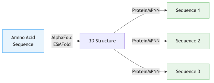
Inverse folding goes the other way. Given a target backbone structure, find amino acid sequences that will fold into it. If AlphaFold is a compiler that turns source code into an executable, ProteinMPNN is a decompiler that recovers source code from the executable.
Forward folding:   MKFLILLFNILCLFPVLAADNH...  -->  3D Structure
                   (AlphaFold, ESMFold)

Inverse folding:   3D Structure  -->  MKFLILLFNILCLFPVLAADNH...
                                  -->  MKYLILIFNLLCLFPVLAADNH...
                                  -->  MRFLILIFNILCLYPVLAADNQ...
                   (ProteinMPNN)       (multiple valid sequences)
Notice a fundamental asymmetry in this diagram. Forward folding typically produces a single dominant structure from a given sequence2. Inverse folding produces many valid sequences for a single structure. This many-to-one mapping is central to understanding why inverse folding is both tractable and useful.
The Many-to-One Mapping
Why can multiple sequences fold into the same structure? The answer lies in the physics of protein folding and the lessons of molecular evolution.
Consider hemoglobin. Human hemoglobin and fish hemoglobin perform the same oxygen-carrying function and adopt remarkably similar three-dimensional structures, yet their sequences can differ by more than 50%. Or consider the immunoglobulin fold—this basic structural motif appears in thousands of different antibody sequences across the immune system, each with unique binding specificity encoded in variable loops but sharing the same underlying architecture.
This sequence tolerance exists because not every amino acid position contributes equally to structural stability. Some positions sit in the hydrophobic core (see Lectures 5-6), where the main requirement is “something nonpolar”—valine, leucine, or isoleucine might all work equally well. Other positions face the solvent and can tolerate almost any hydrophilic residue. Only a subset of positions—those involved in specific hydrogen bonds, salt bridges, or tight packing interactions—are tightly constrained.
Structural biologists quantify this tolerance with sequence identity thresholds (introduced in Preliminary Note 4). Proteins with as little as 20–30% sequence identity often share the same fold. This means roughly 70–80% of positions can vary without disrupting the overall architecture. For inverse folding, this redundancy is a blessing: there is a vast space of valid sequences for any given structure, making the search problem tractable.
ProteinMPNN captures this diversity by learning a conditional probability distribution:
\[P(\mathbf{s} \mid \mathcal{X})\]where \(\mathbf{s} = (s_1, s_2, \dots, s_L)\) is a sequence of \(L\) amino acids and \(\mathcal{X}\) denotes the backbone structure (the set of backbone atom coordinates). Rather than outputting a single “best” sequence, the model provides probabilities for each amino acid at each position, allowing us to sample diverse sequences that are all predicted to fold correctly.
Why Inverse Folding Matters
Inverse folding has become one of the most practically important tools in computational protein design for four reasons.
Completing the design pipeline. Backbone generation methods like RFDiffusion (Lectures 9-10) produce three-dimensional coordinates, but these are not directly manufacturable. Inverse folding provides the missing link, converting geometric designs into genetic sequences that can be ordered as synthetic DNA and expressed in cells.
Sequence optimization. Sometimes you already have a protein that works but could be better—perhaps it expresses poorly in your production system, or it aggregates during purification. Inverse folding can suggest alternative sequences that maintain the same structure while potentially improving biochemical properties like solubility or thermostability.
Exploring sequence space. For a given backbone, inverse folding can generate hundreds of diverse sequences. This is invaluable for experimental screening: you test many variants simultaneously and identify sequences with favorable properties that no single computational method would have predicted.
Understanding evolution. By analyzing which sequence features ProteinMPNN considers important for a given structure, we gain insight into the molecular determinants of protein folding—essentially reverse-engineering nature’s design rules.
2. Why Inverse Design Makes Sense
Nature’s Manufacturing Constraint
Biology does not build proteins from blueprints of atomic coordinates. The cell’s manufacturing machinery—the ribosome—reads a linear genetic message and strings together amino acids one at a time, from the N-terminus to the C-terminus. The resulting polypeptide chain then folds, driven by physics, into a three-dimensional structure. Every protein that has ever existed started as a sequence.
This manufacturing constraint is absolute. No matter how beautiful a backbone structure looks on a computer screen, it cannot be realized in the laboratory without a sequence that encodes it. The inverse folding problem exists because of this constraint: we design in the space of structures (because that is where function lives) but must manufacture in the space of sequences (because that is what biology allows).
Think of it as a bridge problem. On one side: a computational design expressed as three-dimensional coordinates. On the other side: a DNA sequence that can be synthesized for a few hundred dollars and shipped overnight. Inverse folding is the bridge.
Tractability from Redundancy
The many-to-one mapping between sequences and structures might seem like it makes inverse folding harder—a vast search space with no clear starting point. In fact, the opposite is true.
Consider a 100-residue protein. The total number of possible sequences is \(20^{100} \approx 10^{130}\), an incomprehensibly large number. But because roughly 70–80% of positions tolerate multiple amino acids without disrupting the fold, the number of functional sequences—those that fold into the target structure—is enormous. The target is not a needle in a haystack; it is a continent-sized region in sequence space.
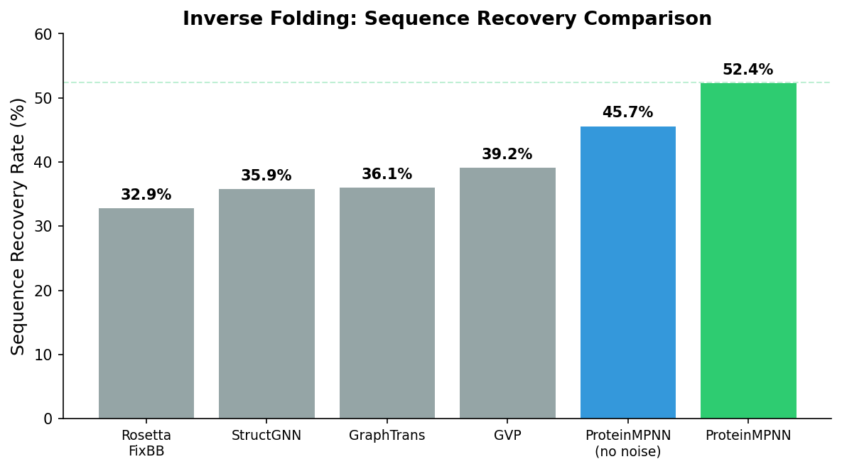
This is why even imperfect methods can find valid sequences. The classic Rosetta fixed-backbone design algorithm, which uses physics-based energy functions and combinatorial optimization, achieved roughly 10% experimental success rates. That 10% was already useful: test 50 sequences, expect 5 to fold correctly. But the margin for error was thin, and many design projects required multiple rounds of iteration.
The 50% Breakthrough
ProteinMPNN changed the calculus. In the original 2022 paper, Dauparas et al. reported that over 50% of designed sequences folded into the target structure when tested experimentally—across a diverse set of protein topologies including helical bundles, beta barrels, and mixed alpha-beta folds. On some protein families, success rates exceeded 70%.
This five-fold improvement over previous methods has two practical consequences. First, fewer sequences need to be tested. Instead of synthesizing 50 candidates and hoping for 5 successes, you can synthesize 10 and expect 5 or more. This cuts the cost and time of experimental validation dramatically. Second, design projects that were previously impractical—those requiring multiple simultaneous successes, such as designing both partners of a protein-protein interaction—become feasible when each component has a high individual success probability.
Speed as a Design Principle
ProteinMPNN generates sequences in seconds on a single GPU. A typical design session produces hundreds of candidate sequences for a given backbone in under a minute. Compare this with physics-based methods like Rosetta, which might require hours of computation per sequence, or with experimental directed evolution, which requires weeks of laboratory work per round.
This speed transforms the design workflow from “carefully craft one sequence and hope it works” to “generate a large diverse pool, filter computationally, and test the best candidates.” The computational cost of inverse folding is negligible compared to every other step in the pipeline: backbone generation, structure prediction for validation, gene synthesis, protein expression, and functional assays. When a step is both fast and accurate, it stops being the bottleneck—and inverse folding has reached that point.
3. How People Solve Protein Design Today
Experimental Success Rates
The 50% headline number from the ProteinMPNN paper is an average across diverse protein topologies. In practice, success rates vary depending on several factors.
Protein size. Small proteins (50–100 residues) tend to have higher success rates than large ones (300+ residues), partly because smaller proteins have fewer opportunities for misfolding and partly because the local structural context captured by ProteinMPNN’s k-nearest-neighbor graph covers a larger fraction of the total structure.
Topology. All-alpha proteins (helical bundles) are generally easier to design than all-beta proteins (beta barrels, beta propellers). Beta sheets impose stricter geometric constraints—hydrogen bond distances and angles must be precise—and ProteinMPNN’s coordinate noise augmentation helps but does not fully compensate. Mixed alpha-beta topologies fall in between.
Solvent exposure. Buried core positions, where the dominant requirement is hydrophobicity, are easier to predict than surface positions, where electrostatic interactions, crystal contacts, and conformational flexibility all contribute. ProteinMPNN achieves the highest sequence recovery rates at buried positions.
Designed vs. natural backbones. ProteinMPNN was trained on natural protein structures from the PDB. Computationally designed backbones from RFDiffusion may contain geometric features not well represented in the training data. Success rates on designed backbones are generally slightly lower than on natural backbones, though still dramatically better than previous methods.
Case Studies
COVID-19 binders. In 2022, the Baker laboratory used the RFDiffusion-ProteinMPNN-AlphaFold pipeline to design de novo protein binders targeting the SARS-CoV-2 spike protein receptor-binding domain. Backbones were generated by RFDiffusion with the spike protein as a target, ProteinMPNN produced candidate sequences, and AlphaFold validated the designs. From design specification to experimentally validated binders with sub-nanomolar affinity took weeks of computation and months of experimental testing—a timeline that would have been years with previous methods.
Enzyme design. Designing enzymes—proteins with catalytic activity—is one of the hardest challenges in protein engineering because catalysis requires precise positioning of reactive residues. Recent work has used ProteinMPNN with fixed catalytic residues (held constant during decoding) to redesign enzyme scaffolds. In several cases, catalytic activity was achieved in the first round of design without directed evolution, something rarely accomplished before.
Protein cages for drug delivery. Symmetric protein assemblies—cages, rings, and fibers—are attractive scaffolds for drug delivery and vaccine design. ProteinMPNN’s tied-position feature ensures that all copies of a symmetric subunit receive the same sequence. Combined with RFDiffusion’s symmetry-aware generation, this has enabled the design of novel protein cages with defined geometry and size.
Receptor traps. Soluble decoy receptors that bind and neutralize inflammatory cytokines are a growing therapeutic modality. ProteinMPNN has been used to redesign natural receptor ectodomains for improved stability and manufacturability while preserving cytokine-binding affinity. The inverse folding step is particularly valuable here because the binding interface is fixed (preserving function) while the scaffold is redesigned (improving biophysical properties).
Practical Tips
How many sequences per backbone? Generate at least 100 candidate sequences per backbone. ProteinMPNN is fast enough that the marginal cost of additional sequences is negligible. More candidates give you better coverage of the viable sequence space and more options after filtering.
Temperature settings. Use a mix of temperatures. Low temperature (\(T = 0.1\)) produces conservative sequences with high predicted confidence—good for maximizing the probability that any single sequence works. Higher temperatures (\(T = 0.3\text{--}1.0\)) produce more diverse sequences that explore a wider range of solutions—good for discovering unexpectedly good designs or for applications where diversity itself is the goal (e.g., antibody library design). A practical split: generate 50 sequences at \(T = 0.1\), 30 at \(T = 0.3\), and 20 at \(T = 1.0\).
Fixed positions vs. full redesign. Fix positions when you have functional constraints: catalytic residues, binding interface residues, disulfide cysteines, or residues at symmetric interfaces. Full redesign (no fixed positions) is appropriate when you want to explore the broadest possible sequence space, such as when designing a protein with no functional requirements beyond folding correctly.
When to use LigandMPNN. LigandMPNN is a variant of ProteinMPNN that is aware of non-protein molecules—small-molecule ligands, metal ions, nucleic acids. Use LigandMPNN when your design includes a bound ligand or cofactor, so that the designed sequence accounts for the interactions at the binding site. Standard ProteinMPNN ignores non-protein atoms entirely.
The role of experimental feedback. Computational protein design is rarely a one-shot process. The first round of designs provides experimental data—which sequences expressed, which folded, which bound the target. This information guides subsequent rounds: adjust the backbone, change fixed positions, modify temperature settings, or switch to a different region of conformational space. Each iteration narrows the design space and improves success rates. The RFDiffusion \(\to\) ProteinMPNN \(\to\) AlphaFold pipeline is fast enough that multiple rounds can be completed in days rather than months.
4. The Design Pipeline: RFDiffusion + ProteinMPNN + AlphaFold
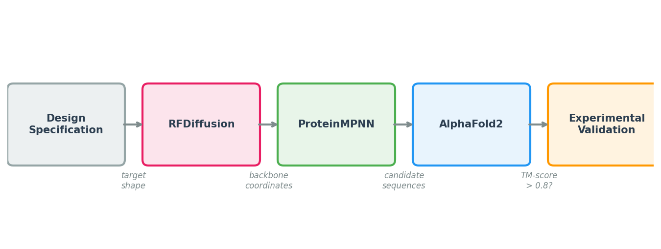

ProteinMPNN’s impact comes from its role in a larger pipeline. No single tool handles the full journey from design specification to experimentally validated protein. The modern computational protein design workflow chains three models together, each solving a different sub-problem.
Step 1: Backbone Generation with RFDiffusion
The pipeline begins with a design specification: a binder to a specific epitope, a symmetric assembly, or an enzyme scaffold with catalytic residues at defined positions. RFDiffusion (Lectures 9-10) takes this specification and generates diverse backbone structures—sets of \((\text{N}, \text{C}_\alpha, \text{C}, \text{O})\) coordinates for each residue—that satisfy the specification.
At this stage, the output is purely geometric. There are no amino acid identities, only a shape.
Step 2: Sequence Design with ProteinMPNN
For each backbone from Step 1, ProteinMPNN generates multiple candidate sequences. Practical recommendations:
- Generate many candidates. ProteinMPNN is fast. Generate 100 or more sequences per backbone, then filter aggressively. The computational cost is negligible compared to the cost of a failed experiment.
- Use multiple temperatures. Generate some sequences at low temperature (\(T = 0.1\), conservative, high confidence) and some at higher temperature (\(T = 0.3\text{--}1.0\), diverse, potentially discovering better solutions). The optimal temperature depends on the application.
- Apply constraints. If certain residues are functionally required (e.g., catalytic triads, disulfide bonds), fix them during decoding.
Step 3: Validation with AlphaFold or ESMFold
The key question is: will the designed sequence actually fold into the intended backbone? To answer this, we run the designed sequence through a structure prediction model—AlphaFold2 (Lectures 7-8) or ESMFold—and compare the predicted structure to the design target.
The primary metric is the TM-score3, which measures global structural similarity on a scale from 0 (unrelated) to 1 (identical). A TM-score above 0.5 generally indicates that two structures share the same fold; designs with TM-scores above 0.8 are considered high-confidence matches. AlphaFold’s per-residue confidence score (pLDDT) provides additional information about which regions of the design are well-predicted.
Step 4: Filtering and Ranking
After structure prediction, filter and rank candidates using:
- TM-score between the predicted and designed backbones.
- pLDDT from AlphaFold (higher is better; values above 80 suggest confident predictions).
- Sequence properties such as predicted solubility, aggregation propensity, and expression likelihood.
- Diversity among the top candidates, to maximize the chance that at least one works experimentally.
Step 5: Experimental Validation
The final step is synthesis and testing. Selected sequences are ordered as synthetic genes, cloned into expression vectors, expressed in cells (typically E. coli or mammalian cell lines), purified, and tested for the intended function.
The original ProteinMPNN paper reported that over 50% of designed sequences folded into the target structure when tested experimentally—a dramatic improvement over previous methods, which achieved roughly 10% success rates. This high hit rate makes the RFDiffusion \(\to\) ProteinMPNN \(\to\) AlphaFold pipeline practical for real-world protein engineering.
Pipeline Summary
Step 1: RFDiffusion
   Specification  -->  Backbone coordinates

Step 2: ProteinMPNN
   Backbone  -->  100+ candidate sequences (diverse temperatures)

Step 3: AlphaFold / ESMFold
   Each sequence  -->  Predicted structure + confidence (pLDDT)

Step 4: Filtering
   Keep sequences where predicted structure matches design (TM-score > 0.8)

Step 5: Experiment
   Synthesize, express, purify, test
Practical Considerations
Consider the full biological context. ProteinMPNN designs sequences for isolated chains or complexes, but the protein will eventually exist inside a cell or in a buffer. Check for protease cleavage sites, glycosylation motifs, and compatibility with your expression system.
Iterate. The pipeline is fast enough to run multiple rounds. If early designs fail, analyze the failures, adjust constraints, and redesign. Each round provides information that improves subsequent attempts.
5. Design Principles and Alternatives
What Makes ProteinMPNN Work
Several design choices contribute to ProteinMPNN’s effectiveness. The table below summarizes them:
| Principle | Implementation | Why It Works |
|---|---|---|
| Structure as graph | k-NN graph on \(\text{C}_\alpha\) atoms | Captures both local and long-range spatial contacts |
| Rich edge features | RBF distances, local frames, orientations | Provides geometric vocabulary beyond raw distances |
| Autoregressive decoding | One amino acid per step | Models inter-residue dependencies accurately |
| Random decoding order | Fresh permutation each training step | Prevents directional bias; enables flexible generation |
| Controlled sampling | Temperature, top-\(k\), top-\(p\) | Balances sequence diversity against design confidence |
Feature Engineering Still Matters
ProteinMPNN’s success relies on carefully designed geometric features—local coordinate frames, RBF-encoded distances, orientation dot products. These features provide the network with a structural vocabulary that would take far more data and capacity to learn from raw coordinates alone. This is an instructive counterpoint to the “end-to-end learning” philosophy: in domains with strong geometric structure, thoughtful feature engineering remains a powerful tool.
Comparison with Alternative Methods
ProteinMPNN is not the only inverse folding method. Understanding the alternatives clarifies its design choices:
| Method | Approach | Key Strength |
|---|---|---|
| ProteinMPNN (Dauparas et al., 2022) | Autoregressive GNN | High accuracy, fast inference, widely adopted |
| ESM-IF (Hsu et al., 2022) | Transformer + ESM language model backbone | Leverages evolutionary knowledge from large-scale pre-training |
| GVP (Jing et al., 2021) | Geometric vector perceptrons | Built-in SE(3) equivariance without data augmentation |
| AlphaDesign | AlphaFold-based end-to-end | Differentiable structure-aware loss |
ProteinMPNN’s combination of accuracy, speed, and simplicity has made it the de facto standard. It runs in seconds per sequence on a single GPU, requires no MSA computation, and integrates seamlessly into the RFDiffusion pipeline.
Key Takeaways
-
Inverse folding converts 3D coordinates to manufacturable amino acid sequences. Proteins are built from sequences, not coordinates. Inverse folding bridges the gap between computational design (in structure space) and biological manufacturing (in sequence space).
-
Many sequences fold into the same structure—a blessing for design. The many-to-one mapping means the space of valid solutions is vast, making the search problem tractable even with imperfect methods.
-
ProteinMPNN achieves over 50% experimental success rate. This five-fold improvement over previous methods (roughly 10%) makes computational protein design practical for real-world applications.
-
The RFDiffusion \(\to\) ProteinMPNN \(\to\) AlphaFold pipeline is the standard workflow. Each model solves a different sub-problem: backbone generation, sequence design, and structure validation.
-
Practical design uses constraints and diversity. Fixed positions preserve functional residues, temperature-controlled sampling balances confidence against exploration, and iterative rounds incorporate experimental feedback.
-
The companion Lecture 12 covers the architecture. Graph construction, message passing, autoregressive decoding, and training—the mechanisms that make ProteinMPNN work.
Code walkthrough: The nano-proteinmpnn walkthrough implements the full architecture from scratch in PyTorch.
-
The name stands for Message Passing Neural Network for Proteins. “Message passing” refers to the graph neural network mechanism at the heart of the model’s structure encoder. ↩
-
In reality, proteins sample an ensemble of conformations, but most well-folded proteins have a single dominant structure that accounts for the vast majority of the ensemble. ↩
-
TM-score stands for Template Modeling score. Unlike RMSD, TM-score is length-normalized and less sensitive to local structural deviations, making it a better metric for assessing overall fold similarity. ↩