RFDiffusion: SE(3) Diffusion for Protein Backbones
This is Lecture 10 of the Protein & Artificial Intelligence course (Spring 2026), co-taught by Prof. Sungsoo Ahn and Prof. Homin Kim at KAIST. This is the most mathematically intensive lecture in the course: it requires careful treatment of Lie groups, manifold-valued noise processes, and equivariant neural network design. It serves as the implementation companion to Lecture 9 (Protein Backbone Design) and builds on diffusion model foundations from Lecture 4 and structure prediction concepts from Lecture 8.
Introduction
Lecture 9 framed the protein backbone design problem and showed why controlling three-dimensional shape gives control over biological function. It surveyed the practical design pipeline — RFDiffusion for backbone generation, ProteinMPNN for sequence design, AlphaFold2 for validation — and catalogued the experimental successes: novel folds, functional binders, symmetric assemblies.
This lecture develops the mathematical and computational machinery underneath. The central questions are: how do you represent protein geometry in a way that respects physical symmetry? how do you define noise on a curved manifold of rotations? and how do you build a neural network that generates protein backbones while satisfying SE(3) equivariance by construction?
The answers draw on Lie group theory (\(SO(3)\) and \(SE(3)\)), differential geometry (the IGSO(3) distribution as a Gaussian analogue on a manifold), and equivariant neural network design (invariant features, local-frame updates). The reward is a generative model that produces physically valid protein geometries at every step, without post-hoc corrections.
Roadmap
| Section | Topic | Why It Is Needed |
|---|---|---|
| 1 | SE(3) equivariance | Proteins are geometric objects; a model that ignores this wastes data and generalizes poorly |
| 2 | Rotation representations | Before diffusing rotations, we need a numerically stable way to represent them |
| 3 | Frame representation | Each residue is a rigid body; frames are the natural state space for protein backbones |
| 4 | IGSO(3) distribution | Standard Gaussian noise is undefined on the rotation manifold; IGSO(3) fills this gap |
| 5 | SE(3) diffusion process | Combining translational and rotational noise into a single forward process |
| 6 | Equivariant neural networks | The denoiser must respect SE(3) symmetry by construction |
| 7 | RFDiffusion architecture | How RoseTTAFold is adapted from structure prediction to structure generation |
| 8 | Conditional generation | Implementation of motif scaffolding, self-conditioning, and classifier-free guidance |
| 9 | Training and loss functions | How the model learns to denoise on SE(3) |
| 10 | Sampling and generation | The reverse process that produces novel protein backbones |
1. Why Geometry Matters: The Case for SE(3) Equivariance
Proteins Do Not Have a Preferred Orientation
Suppose you determine the crystal structure of an enzyme. You record the coordinates of every atom. Now a colleague in another laboratory solves the same structure, but their crystal happened to grow in a different orientation. Their coordinates differ from yours by a rotation and a translation, yet the two structures are identical in every biological sense. The enzyme catalyzes the same reaction. Its binding affinity for a substrate is unchanged. Its stability is the same.
This observation has a name: the biological properties of a protein are invariant under the group of rigid-body transformations in three-dimensional space. That group is called \(SE(3)\), the Special Euclidean group in three dimensions1. An element of \(SE(3)\) is a pair \((R, \vec{t})\) where \(R\) is a \(3 \times 3\) rotation matrix and \(\vec{t}\) is a translation vector in \(\mathbb{R}^3\). It acts on a point \(\vec{x} \in \mathbb{R}^3\) by
\[T \cdot \vec{x} = R\vec{x} + \vec{t}.\]From Invariance to Equivariance
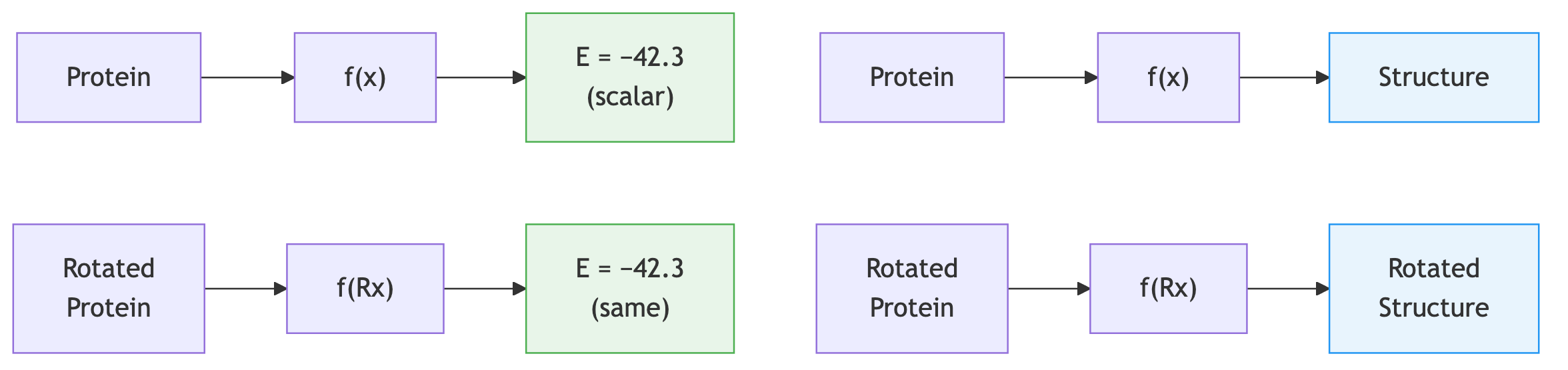
Invariance tells us what properties should not change under transformations. But a generative model does not just compute scalar properties — it outputs structures, which are geometric objects that should transform when the input transforms.
If you rotate the conditioning information fed to a protein generator, the generated structure should rotate by the same amount. This stronger requirement is called SE(3) equivariance. A function \(f\) is equivariant with respect to a group \(G\) if, for every group element \(g \in G\),
\[f(g \cdot x) = g \cdot f(x).\]In words: applying the transformation before the function gives the same result as applying it after.
Why Not Just Augment the Data?
A natural objection is: why build equivariance into the architecture when we could simply augment the training data with random rotations and translations?
Data augmentation does help, but it has three limitations compared to architectural equivariance.
Data efficiency. An equivariant model knows, by construction, that all orientations of a protein are equivalent. It never needs to “learn” this from examples. A non-equivariant model must see the same structure from many orientations before it generalizes, which wastes precious training data.
Guaranteed generalization. No amount of data augmentation can guarantee that a model has perfectly learned the symmetry. An equivariant architecture satisfies the symmetry exactly, for every possible input, including inputs far from the training distribution.
Physically meaningful representations. When a model is equivariant, its internal feature vectors have well-defined transformation laws. Vectors transform like vectors; scalars remain scalars. This makes the representations more interpretable and more likely to capture physically meaningful relationships.
2. The Language of Rotations
Before adding noise to the orientation of a protein residue, we need a concrete way to represent rotations. This turns out to be more subtle than it first appears, and the choice of representation has significant consequences for numerical stability.
A rotation in three dimensions has three degrees of freedom. The three angles needed to orient a rigid body: pitch, yaw, and roll. Yet the four most common representations use different numbers of parameters.
Rotation Matrices
A rotation is a \(3 \times 3\) orthogonal matrix \(R\) with determinant \(+1\). It acts on a vector \(\vec{v}\) by matrix multiplication: \(\vec{v}' = R\vec{v}\). The set of all such matrices forms the group \(SO(3)\)2.
Rotation matrices are direct and easy to compose (matrix multiplication), but they use nine numbers to describe three degrees of freedom. The six constraints (orthogonality and unit determinant) must be enforced explicitly, which can cause numerical drift in iterative algorithms.
Euler Angles
Three angles \((\phi, \theta, \psi)\) describe successive rotations about coordinate axes. This representation is minimal (three numbers for three degrees of freedom) and intuitive, but it suffers from gimbal lock: at certain orientations, two of the three axes align, and the representation loses a degree of freedom. Gimbal lock causes discontinuities that are catastrophic for gradient-based optimization.
Axis-Angle Representation
Any rotation can be described by a unit vector \(\hat{n}\) (the axis) and a scalar \(\omega\) (the angle). The combined representation \(\vec{\omega} = \omega \hat{n}\) is a three-dimensional vector whose direction is the rotation axis and whose magnitude is the rotation angle.
This representation is minimal and geometrically intuitive. The axis-angle representation lives in a tangent space — a flat approximation of the curved rotation space near the identity rotation. Mathematicians call this tangent space the Lie algebra \(\mathfrak{so}(3)\), and it will be important when we define noise processes. Its main drawback is a singularity at \(\omega = 0\), where the axis is undefined.
The conversion from axis-angle to rotation matrix uses the Rodrigues formula:
\[R = I + \sin(\omega) K + (1 - \cos(\omega)) K^2,\]where \(K\) is the skew-symmetric matrix constructed from the axis vector \(\hat{n}\), and \(I\) is the \(3 \times 3\) identity matrix3.
import torch
import numpy as np

def skew_symmetric(v):
    """
    Construct the 3x3 skew-symmetric matrix [v]_x from a 3D vector v.

    For a vector v = (v1, v2, v3), the skew-symmetric matrix satisfies
    [v]_x @ w = v x w (cross product) for any vector w.

    Args:
        v: [..., 3] axis vectors (e.g., rotation axes for each residue)

    Returns:
        K: [..., 3, 3] skew-symmetric matrices
    """
    batch_shape = v.shape[:-1]
    zero = torch.zeros(*batch_shape, device=v.device)

    return torch.stack([
        torch.stack([zero,    -v[..., 2],  v[..., 1]], dim=-1),
        torch.stack([v[..., 2],  zero,    -v[..., 0]], dim=-1),
        torch.stack([-v[..., 1], v[..., 0],  zero   ], dim=-1)
    ], dim=-2)


def axis_angle_to_rotation_matrix(axis_angle):
    """
    Convert axis-angle vectors to rotation matrices via the Rodrigues formula.

    Each residue's orientation perturbation can be expressed as a rotation
    by angle omega about axis n_hat. This function converts that compact
    representation into the full 3x3 matrix needed for coordinate transforms.

    Args:
        axis_angle: [..., 3] vectors where direction = axis, magnitude = angle

    Returns:
        R: [..., 3, 3] rotation matrices
    """
    angle = axis_angle.norm(dim=-1, keepdim=True)  # rotation angle omega
    axis = axis_angle / (angle + 1e-8)              # unit axis n_hat

    K = skew_symmetric(axis)  # [..., 3, 3]

    I = torch.eye(3, device=axis_angle.device).expand(
        *axis_angle.shape[:-1], 3, 3
    )
    sin_angle = torch.sin(angle).unsqueeze(-1)
    cos_angle = torch.cos(angle).unsqueeze(-1)

    # Rodrigues: R = I + sin(omega) * K + (1 - cos(omega)) * K^2
    R = I + sin_angle * K + (1 - cos_angle) * torch.einsum(
        '...ij,...jk->...ik', K, K
    )
    return R
Quaternions
A unit quaternion \(q = (w, x, y, z)\) with \(w^2 + x^2 + y^2 + z^2 = 1\) provides a four-parameter representation of a rotation. The extra parameter (four instead of three) buys important benefits: quaternions are free of singularities, interpolate smoothly, and compose efficiently. They also have a double-cover property — \(q\) and \(-q\) represent the same rotation — which must be handled carefully but is not a practical obstacle.
RFDiffusion uses quaternions internally for numerical stability. The conversion between quaternions and rotation matrices:
def quaternion_to_rotation_matrix(q):
    """
    Convert unit quaternions to rotation matrices.

    Quaternions avoid gimbal lock and provide numerically stable
    interpolation between orientations --- critical when iteratively
    updating residue frames during diffusion.

    Args:
        q: [..., 4] quaternions in (w, x, y, z) convention

    Returns:
        R: [..., 3, 3] rotation matrices
    """
    # Normalize to unit quaternion (guards against numerical drift)
    q = q / (q.norm(dim=-1, keepdim=True) + 1e-8)
    w, x, y, z = q.unbind(-1)

    R = torch.stack([
        torch.stack([1 - 2*y*y - 2*z*z, 2*x*y - 2*w*z, 2*x*z + 2*w*y], dim=-1),
        torch.stack([2*x*y + 2*w*z, 1 - 2*x*x - 2*z*z, 2*y*z - 2*w*x], dim=-1),
        torch.stack([2*x*z - 2*w*y, 2*y*z + 2*w*x, 1 - 2*x*x - 2*y*y], dim=-1)
    ], dim=-2)
    return R


def rotation_matrix_to_quaternion(R):
    """
    Convert rotation matrices to unit quaternions.

    This uses the Shepperd method based on the matrix trace. The
    implementation handles the common case where the trace is positive;
    production code should also handle degenerate cases.

    Args:
        R: [..., 3, 3] rotation matrices

    Returns:
        q: [..., 4] unit quaternions (w, x, y, z)
    """
    trace = R[..., 0, 0] + R[..., 1, 1] + R[..., 2, 2]

    w = torch.sqrt(torch.clamp(1 + trace, min=1e-8)) / 2
    x = (R[..., 2, 1] - R[..., 1, 2]) / (4 * w + 1e-8)
    y = (R[..., 0, 2] - R[..., 2, 0]) / (4 * w + 1e-8)
    z = (R[..., 1, 0] - R[..., 0, 1]) / (4 * w + 1e-8)

    q = torch.stack([w, x, y, z], dim=-1)
    return q / (q.norm(dim=-1, keepdim=True) + 1e-8)
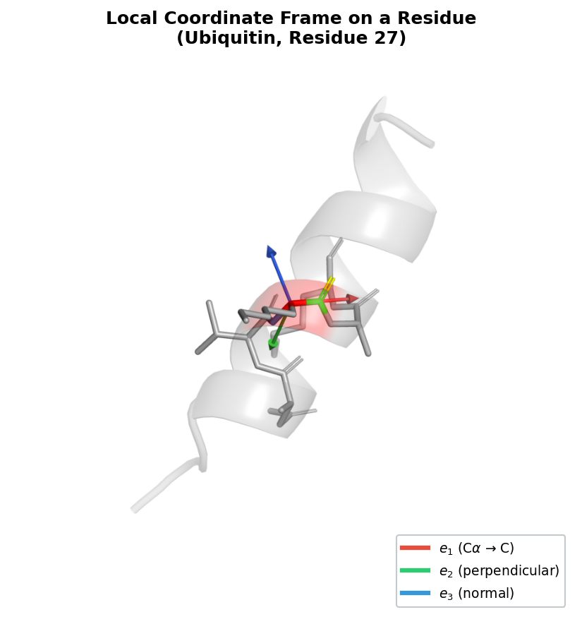
3. Each Amino Acid Has Its Own Coordinate System
The Frame Representation
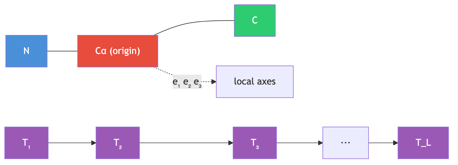
A protein backbone4 consists of a chain of amino acid residues. Each residue contains three backbone atoms — nitrogen (N), alpha carbon (\(\text{C}_\alpha\)), and carbonyl carbon (C) — that form a relatively rigid unit5.
Two pieces of information fully specify the placement of this unit in space:
- Position: the location of the \(\text{C}_\alpha\) atom, a vector \(\vec{t}_i \in \mathbb{R}^3\).
- Orientation: the direction the residue “faces,” encoded as a rotation matrix \(R_i \in SO(3)\) that maps from a canonical local coordinate system to the global frame.

The three dihedral angles6 \(\phi\), \(\psi\), and \(\omega\) specify the backbone conformation at each residue.
Together, the pair \((R_i, \vec{t}_i)\) defines a rigid-body frame for residue \(i\).
The set of all such pairs forms the group \(SE(3)\): a transformation \(T = (R, \vec{t})\) acts on a point \(\vec{x}\) by
\[T \cdot \vec{x} = R\vec{x} + \vec{t}.\]A protein backbone with \(L\) residues is therefore a sequence of \(L\) frames:
\[\mathcal{T} = \{T_1, T_2, \ldots, T_L\}, \quad T_i = (R_i, \vec{t}_i) \in SE(3).\]This representation is powerful for three reasons. First, it is complete: given all \(L\) frames plus the amino acid identities, we can reconstruct the full atomic structure (backbone atoms are placed by the frame; side-chain atoms are placed by the identity and local geometry). Second, it is compact: only \(6L\) degrees of freedom (three for position, three for orientation, per residue). Third, it is geometrically natural: the relative transformation between two frames, \(T_i^{-1} \circ T_j\), captures the intrinsic geometry of the residue pair independent of global orientation.
Implementation
class RigidTransform:
    """
    Rigid body transformation (rotation + translation) for protein residues.

    Each residue in a protein backbone is described by a frame T = (R, t),
    where R is a 3x3 rotation matrix defining the local coordinate system
    and t is a 3D vector giving the C-alpha position.
    """

    def __init__(self, rotations, translations):
        """
        Args:
            rotations:    [..., 3, 3] rotation matrices (one per residue)
            translations: [..., 3]    C-alpha positions (one per residue)
        """
        self.rots = rotations
        self.trans = translations

    @classmethod
    def identity(cls, batch_shape, device='cpu'):
        """Create identity frames (no rotation, origin position)."""
        rots = torch.eye(3, device=device).expand(*batch_shape, 3, 3).clone()
        trans = torch.zeros(*batch_shape, 3, device=device)
        return cls(rots, trans)

    def compose(self, other):
        """
        Compose two transformations: self followed by other.
        Result: (R1 @ R2, R1 @ t2 + t1)
        """
        new_rots = torch.einsum('...ij,...jk->...ik', self.rots, other.rots)
        new_trans = (
            torch.einsum('...ij,...j->...i', self.rots, other.trans)
            + self.trans
        )
        return RigidTransform(new_rots, new_trans)

    def apply(self, points):
        """Apply transformation to points: R @ x + t."""
        return (
            torch.einsum('...ij,...j->...i', self.rots, points) + self.trans
        )

    def invert(self):
        """Compute inverse transformation: (R^T, -R^T @ t)."""
        inv_rots = self.rots.transpose(-1, -2)
        inv_trans = -torch.einsum('...ij,...j->...i', inv_rots, self.trans)
        return RigidTransform(inv_rots, inv_trans)

    def to_tensor_7(self):
        """Convert to 7D representation (quaternion + translation)."""
        quat = rotation_matrix_to_quaternion(self.rots)
        return torch.cat([quat, self.trans], dim=-1)

    @classmethod
    def from_tensor_7(cls, tensor):
        """Create from 7D representation (quaternion + translation)."""
        quat = tensor[..., :4]
        trans = tensor[..., 4:]
        rots = quaternion_to_rotation_matrix(quat)
        return cls(rots, trans)
The compose method deserves special attention. When we compose two rigid-body transformations \(T_1 = (R_1, \vec{t}_1)\) and \(T_2 = (R_2, \vec{t}_2)\), the result is
This is not commutative: \(T_1 \circ T_2 \neq T_2 \circ T_1\) in general. The order matters because rotations are applied to subsequent translations. This non-commutativity is a fundamental feature of \(SE(3)\) and has direct consequences for how we apply frame updates during denoising.
4. Diffusion Meets Geometry: The IGSO(3) Distribution
The Challenge of Adding Noise to Rotations
Recall from Lecture 4 (Diffusion Models) how standard diffusion works for data in Euclidean space. Given a clean data point \(x_0\), we define a forward process that gradually adds Gaussian noise:
\[x_t = \sqrt{\bar{\alpha}_t} \, x_0 + \sqrt{1 - \bar{\alpha}_t} \, \epsilon, \quad \epsilon \sim \mathcal{N}(0, I),\]where \(\bar{\alpha}_t\) is a noise schedule parameter that decreases from 1 (clean) to 0 (pure noise) as the timestep \(t\) increases.
This works perfectly for the translational component of protein frames — positions \(\vec{t}_i\) live in \(\mathbb{R}^3\), and Gaussian noise in \(\mathbb{R}^3\) is well defined.
But rotations live on a manifold7 — a space that is locally flat (like a small patch of a sphere looks flat) but globally curved.
You cannot “add” Gaussian noise to a rotation matrix and expect the result to remain a valid rotation. The matrix \(R + \epsilon\) (with \(\epsilon\) drawn from a matrix-valued Gaussian) is not orthogonal, does not have determinant one, and does not represent a rotation at all.
A noise distribution native to the rotation manifold is needed.
The Isotropic Gaussian on SO(3)
The solution is the Isotropic Gaussian distribution on SO(3), abbreviated IGSO(3)8. This distribution plays the same role for rotations that the standard Gaussian plays for Euclidean data: it provides a way to add controlled, isotropic9 noise
Here is the intuition. Imagine holding a pointer that starts aimed at the north pole of a sphere. A sample from IGSO(3) with parameter \(\sigma\) rotates this pointer by a random angle \(\omega\) drawn from a distribution that is approximately Gaussian with standard deviation \(\sigma\), around a uniformly random axis.
- When \(\sigma\) is small, the perturbation is small: the pointer stays near the north pole.
- When \(\sigma\) is large, the pointer can end up anywhere on the sphere.
- In the limit \(\sigma \to \infty\), the distribution becomes the uniform (Haar) measure over \(SO(3)\): every orientation is equally likely.
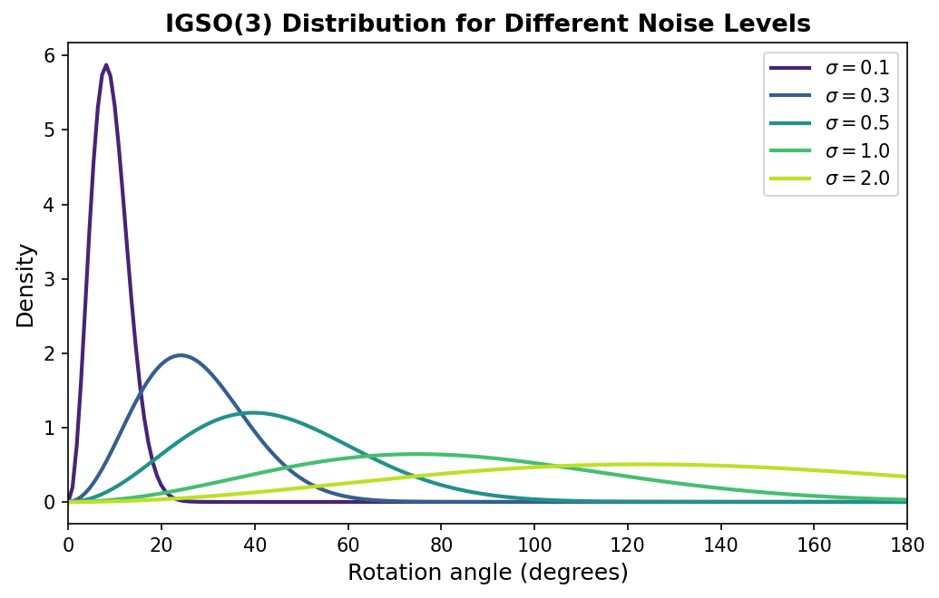
Formally, the density of IGSO(3) with concentration parameter \(\sigma\) at a rotation \(R\) is
\[p(R \mid \sigma) \propto \sum_{\ell=0}^{\infty} (2\ell + 1) \exp\!\left(-\frac{\ell(\ell+1)\sigma^2}{2}\right) \chi_\ell(R),\]where \(\chi_\ell(R)\) is the character of the irreducible representation of \(SO(3)\) at degree \(\ell\)10. In practice, for the rotation angles relevant to protein diffusion, this is well approximated by a simpler expression that depends only on the rotation angle \(\omega\) of \(R\):
\[p(\omega \mid \sigma) \propto (1 - \cos \omega) \exp\!\left(-\frac{\omega^2}{2\sigma^2}\right).\]The \((1 - \cos \omega)\) factor accounts for the geometry of the rotation space — just as the surface area element of a sphere requires a \(\sin\theta\) factor, the “volume element” of \(SO(3)\) requires this correction. This geometric correction factor is called the Haar measure density on \(SO(3)\), expressed in the angle variable.
Sampling from IGSO(3)
Sampling from IGSO(3) is straightforward using the axis-angle decomposition:
- Draw a rotation angle \(\omega\) from a folded normal distribution with standard deviation \(\sigma\).
- Draw a rotation axis \(\hat{n}\) uniformly from the unit sphere \(S^2\).
- Convert the axis-angle pair \((\hat{n}, \omega)\) to a rotation matrix using the Rodrigues formula.
def sample_igso3(shape, sigma, device='cpu'):
    """
    Sample rotation matrices from the Isotropic Gaussian on SO(3).

    This is the rotational analogue of sampling from a Gaussian in
    Euclidean space. Each sample is a random rotation whose angle
    (roughly) follows a Gaussian with standard deviation sigma,
    applied about a uniformly random axis.

    Args:
        shape:  batch dimensions (e.g., (L,) for L residues)
        sigma:  noise level (scalar or broadcastable tensor);
                small sigma -> small perturbations, large sigma -> near-uniform
        device: torch device

    Returns:
        rotations: [*shape, 3, 3] sampled rotation matrices
    """
    # Step 1: Sample rotation angle |omega| ~ folded normal(0, sigma^2)
    omega = torch.abs(torch.randn(*shape, device=device) * sigma)

    # Step 2: Sample rotation axis uniformly on the unit sphere S^2
    axis = torch.randn(*shape, 3, device=device)
    axis = axis / (axis.norm(dim=-1, keepdim=True) + 1e-8)

    # Step 3: Convert to rotation matrix via Rodrigues formula
    rotations = axis_angle_to_rotation_matrix(axis * omega.unsqueeze(-1))

    return rotations
The key property of this sampling procedure is that the resulting distribution is isotropic: it treats all rotation axes equally. There is no preferred direction of perturbation, just as standard Gaussian noise in \(\mathbb{R}^3\) treats all spatial directions equally.
5. The Complete SE(3) Diffusion Process
With the IGSO(3) distribution in hand, the full forward diffusion process for protein frames treats the translational and rotational components separately, using the appropriate noise distribution for each.
Translational Diffusion
Translations live in \(\mathbb{R}^3\), so standard Gaussian diffusion applies directly. Given clean \(\text{C}_\alpha\) positions \(\vec{t}_0\) and a noise schedule parameter \(\bar{\alpha}_t\):
\[\vec{t}_t = \sqrt{\bar{\alpha}_t} \, \vec{t}_0 + \sqrt{1 - \bar{\alpha}_t} \, \epsilon, \quad \epsilon \sim \mathcal{N}(0, I).\]def diffuse_translations(translations, t, noise_schedule):
"""
Add Gaussian noise to C-alpha positions.
Args:
translations: [..., 3] clean C-alpha positions
t: [...] diffusion timesteps in [0, 1]
noise_schedule: object providing alpha_bar(t)
Returns:
noisy_translations: [..., 3]
noise: [..., 3] the sampled Gaussian noise
"""
alpha_bar = noise_schedule.alpha_bar(t) # [..., 1]
noise = torch.randn_like(translations)
noisy = torch.sqrt(alpha_bar) * translations + torch.sqrt(1 - alpha_bar) * noise
return noisy, noise
Rotational Diffusion
Rotations live on \(SO(3)\), so IGSO(3) is used instead. Given a clean rotation \(R_0\) and a noise level \(\sigma_t\), the noisy rotation is obtained by composing \(R_0\) with a random rotation sampled from IGSO(3):
\[R_t = R_{\text{noise}} \cdot R_0, \quad R_{\text{noise}} \sim \text{IGSO}(3; \sigma_t).\]Composition (matrix multiplication) replaces addition because \(SO(3)\) is a group, not a vector space. The noise rotation \(R_{\text{noise}}\) acts as a random perturbation applied to the clean orientation.
def diffuse_rotations(rotations, t, noise_schedule):
    """
    Add IGSO(3) noise to residue orientations.

    Unlike translations (where noise is added), rotational noise is
    composed (multiplied) because SO(3) is a multiplicative group.

    Args:
        rotations:      [..., 3, 3] clean rotation matrices
        t:              [...] diffusion timesteps in [0, 1]
        noise_schedule: object providing sigma_rot(t)

    Returns:
        noisy_rotations: [..., 3, 3]
        noise_rotations: [..., 3, 3] the IGSO(3) samples that were applied
    """
    sigma = noise_schedule.sigma_rot(t)

    # Sample noise rotation from IGSO(3)
    noise_rot = sample_igso3(rotations.shape[:-2], sigma, rotations.device)

    # Compose: R_t = R_noise @ R_0
    noisy_rotations = torch.einsum('...ij,...jk->...ik', noise_rot, rotations)

    return noisy_rotations, noise_rot
The Noise Schedule
The noise schedule controls how quickly the signal is destroyed during the forward process. RFDiffusion uses a cosine schedule for translations (which produces a smooth transition from clean to noisy) and a linear schedule for rotations:
class SE3DiffusionSchedule:
    """
    Noise schedule for SE(3) diffusion on protein frames.

    The translation schedule uses the cosine form from Nichol & Dhariwal (2021),
    which avoids the abrupt noise increase at the end of a linear schedule.
    The rotation schedule is linear in the IGSO(3) concentration parameter.
    """

    def __init__(self, T=1000, trans_sigma_max=10.0, rot_sigma_max=1.5):
        """
        Args:
            T:              number of diffusion timesteps
            trans_sigma_max: maximum translation noise (Angstroms)
            rot_sigma_max:  maximum rotation noise (radians, roughly)
        """
        self.T = T
        self.trans_sigma_max = trans_sigma_max
        self.rot_sigma_max = rot_sigma_max

    def alpha_bar(self, t):
        """Cosine schedule for translations: alpha_bar(t) in [0, 1]."""
        s = 0.008  # small offset to prevent alpha_bar(0) = 1 exactly
        f_t = torch.cos((t + s) / (1 + s) * np.pi / 2) ** 2
        f_0 = np.cos(s / (1 + s) * np.pi / 2) ** 2
        return f_t / f_0

    def sigma_rot(self, t):
        """Linear schedule for rotations: sigma(t) = t * sigma_max."""
        return t * self.rot_sigma_max

    def sample_timestep(self, batch_size, device='cpu'):
        """Sample uniform random timesteps in [0, 1]."""
        return torch.rand(batch_size, device=device)
Combining Both Components
The full forward process diffuses translations and rotations jointly:
def diffuse_frames(frames, t, schedule):
    """
    Apply the SE(3) forward diffusion process to protein frames.

    Each residue frame T_i = (R_i, t_i) is independently noised:
    - Positions receive Gaussian noise in R^3
    - Orientations receive IGSO(3) noise on SO(3)

    Args:
        frames:   RigidTransform with L residue frames
        t:        [L] or scalar timestep
        schedule: SE3DiffusionSchedule

    Returns:
        noisy_frames: RigidTransform (the noised structure)
        noise:        dict with 'trans' and 'rot' noise components
    """
    noisy_trans, trans_noise = diffuse_translations(
        frames.trans, t.unsqueeze(-1), schedule
    )
    noisy_rots, rot_noise = diffuse_rotations(
        frames.rots, t, schedule
    )

    noisy_frames = RigidTransform(noisy_rots, noisy_trans)
    noise = {'trans': trans_noise, 'rot': rot_noise}
    return noisy_frames, noise
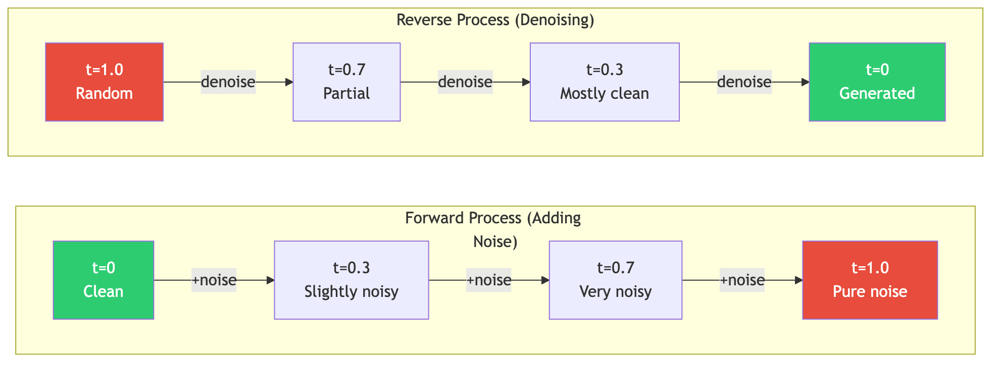
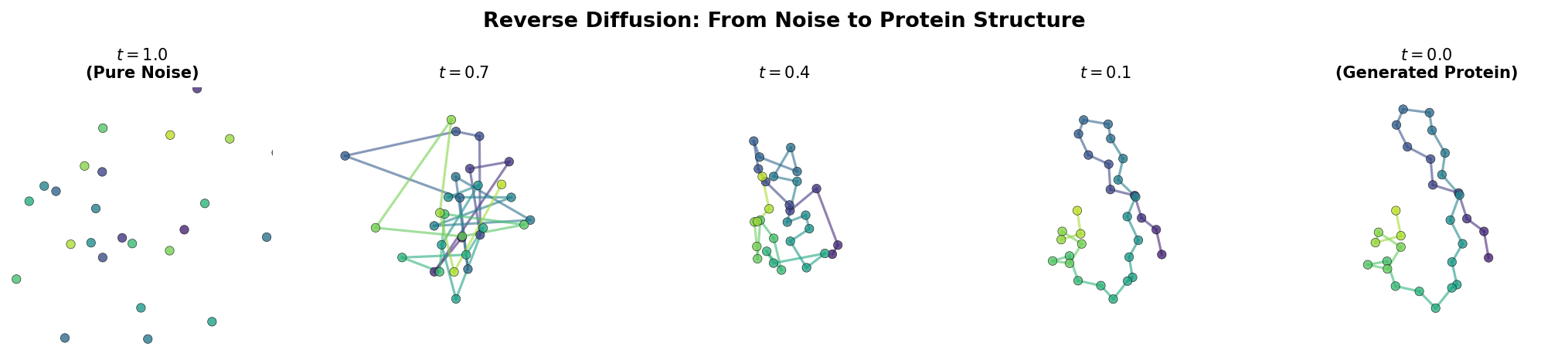
At \(t = 0\), the frames are clean. At \(t = 1\), the positions are nearly pure Gaussian noise and the orientations are nearly uniformly random. The neural network’s job is to learn the reverse of this process: given a noisy structure and the noise level, predict the clean structure.
6. Building Equivariant Neural Networks
The Core Principle
The denoiser takes noisy protein frames and produces denoised frames, while satisfying SE(3) equivariance. The design principle is:
Compute using invariant features. Apply results in local coordinate frames.
Invariant features are quantities that do not change when the entire protein is rotated or translated. Examples include distances between \(\text{C}_\alpha\) atoms, angles between bonds, and the relative rotation angle between two residue frames. These features are “safe” inputs to any standard neural network layer (MLPs, attention, etc.) because they carry no orientation information.
The outputs of the network — frame updates — are predicted in each residue’s local coordinate frame and then transformed to global coordinates using the residue’s rotation matrix. Because the local frame rotates with the protein, the global output rotates correctly.
Invariant Edge Features
The first step is to compute invariant features for each pair of interacting residues:
def compute_invariant_edge_features(frames, edge_index, max_dist=20.0):
    """
    Compute SE(3)-invariant features for pairs of residues.

    These features describe the geometric relationship between two
    residues without reference to any global coordinate system.

    Args:
        frames:    RigidTransform [N] (one frame per residue)
        edge_index: [2, E] pairs of interacting residues
        max_dist:  maximum distance for radial basis encoding (Angstroms)

    Returns:
        edge_features: [E, edge_dim] invariant features
    """
    src, dst = edge_index

    # --- Distance (invariant under all of SE(3)) ---
    pos_src = frames.trans[src]
    pos_dst = frames.trans[dst]
    distances = (pos_src - pos_dst).norm(dim=-1, keepdim=True)

    # Encode distance with radial basis functions
    rbf_dist = rbf_encode(distances, n_bins=16, max_val=max_dist)

    # --- Relative rotation angle (invariant under global rotation) ---
    # R_rel = R_dst^T @ R_src captures how one frame is rotated
    # relative to the other, independent of global orientation.
    R_rel = torch.einsum(
        'eij,ejk->eik',
        frames.rots[dst].transpose(-1, -2),
        frames.rots[src]
    )
    trace = R_rel[:, 0, 0] + R_rel[:, 1, 1] + R_rel[:, 2, 2]
    rot_angle = torch.acos(torch.clamp((trace - 1) / 2, -1, 1))

    # Combine into feature vector
    edge_features = torch.cat([
        rbf_dist,
        rot_angle.unsqueeze(-1),
        torch.sin(rot_angle).unsqueeze(-1),
        torch.cos(rot_angle).unsqueeze(-1)
    ], dim=-1)

    return edge_features


def rbf_encode(distances, n_bins=16, max_val=20.0):
    """
    Radial basis function encoding of distances.

    Transforms a scalar distance into a vector of Gaussian bumps centered
    at evenly spaced values. This gives the network a richer representation
    of distance than a single scalar.

    Args:
        distances: [..., 1] pairwise distances in Angstroms
        n_bins:    number of Gaussian basis functions
        max_val:   maximum distance to encode

    Returns:
        rbf: [..., n_bins] encoded distances
    """
    centers = torch.linspace(0, max_val, n_bins, device=distances.device)
    gamma = 1.0 / (max_val / n_bins)
    return torch.exp(-gamma * (distances - centers) ** 2)
The relative rotation angle \(\omega_{ij}\) between residues \(i\) and \(j\) is computed from the trace of the relative rotation matrix \(R_j^T R_i\). The trace of a rotation matrix is \(1 + 2\cos\omega\), so \(\omega = \arccos\!\bigl(\frac{\text{tr}(R_j^T R_i) - 1}{2}\bigr)\). This angle is invariant: rotating the entire protein changes both \(R_i\) and \(R_j\) by the same global rotation, which cancels in the product \(R_j^T R_i\).
An Equivariant Convolution Layer
With invariant edge features in hand, a message-passing layer updates both node features and positions equivariantly:
class SE3EquivariantConv(nn.Module):
    """
    SE(3)-equivariant graph convolution layer for protein residues.

    Messages between residues are computed from invariant features
    (distances, relative orientations). Position updates are predicted
    in the local coordinate frame of each source residue, then
    transformed to global coordinates. This ensures equivariance:
    rotating the input rotates the output by the same amount.
    """

    def __init__(self, node_dim, edge_dim, hidden_dim=128):
        super().__init__()
        self.node_dim = node_dim
        self.edge_dim = edge_dim

        # Process invariant edge features
        self.edge_mlp = nn.Sequential(
            nn.Linear(edge_dim, hidden_dim),
            nn.ReLU(),
            nn.Linear(hidden_dim, hidden_dim)
        )

        # Compute scalar messages (invariant)
        self.message_mlp = nn.Sequential(
            nn.Linear(node_dim * 2 + hidden_dim, hidden_dim),
            nn.ReLU(),
            nn.Linear(hidden_dim, node_dim)
        )

        # Predict position displacements in local frames (equivariant)
        self.pos_mlp = nn.Sequential(
            nn.Linear(node_dim * 2 + hidden_dim, hidden_dim),
            nn.ReLU(),
            nn.Linear(hidden_dim, 3)
        )

    def forward(self, node_features, frames, edge_index, edge_features):
        """
        Args:
            node_features: [N, node_dim] per-residue features
            frames:        RigidTransform [N] per-residue frames
            edge_index:    [2, E] edges (pairs of interacting residues)
            edge_features: [E, edge_dim] invariant edge features

        Returns:
            updated_features:  [N, node_dim] updated per-residue features
            position_updates:  [N, 3] equivariant position updates
        """
        src, dst = edge_index
        N = node_features.shape[0]

        # Embed edge features
        edge_emb = self.edge_mlp(edge_features)

        # Build message inputs
        src_feat = node_features[src]
        dst_feat = node_features[dst]
        msg_input = torch.cat([src_feat, dst_feat, edge_emb], dim=-1)

        # Compute scalar messages and aggregate
        messages = self.message_mlp(msg_input)
        agg = torch.zeros(N, self.node_dim, device=messages.device)
        agg.scatter_add_(0, dst.unsqueeze(-1).expand(-1, self.node_dim), messages)

        # Predict position updates in SOURCE residue's local frame
        pos_local = self.pos_mlp(msg_input)  # [E, 3]

        # Transform to global coordinates using source frame's rotation
        src_frames = RigidTransform(frames.rots[src], frames.trans[src])
        pos_global = src_frames.apply(pos_local) - src_frames.trans

        # Aggregate position updates at destination residues
        pos_agg = torch.zeros(N, 3, device=pos_global.device)
        pos_agg.scatter_add_(0, dst.unsqueeze(-1).expand(-1, 3), pos_global)

        return node_features + agg, pos_agg
The equivariance guarantee comes from the position update pathway. The MLP receives only invariant inputs and produces a 3D vector in the local coordinate frame of the source residue. When the entire protein is rotated by \(R_g\), the source frame’s rotation becomes \(R_g R_i\), and the global update becomes \(R_g R_i \vec{d} = R_g (R_i \vec{d})\) — the original global update rotated by \(R_g\). This is exactly the equivariance condition.
7. The RFDiffusion Architecture
From Structure Prediction to Structure Generation
RFDiffusion does not build its neural network from scratch. Instead, it adapts the architecture of RoseTTAFold [b], a protein structure prediction model, for the generative task. This strategy has two advantages: the pretrained weights provide a strong initialization, and the architecture is already designed to process protein geometry.
The high-level flow is:
- Input: noisy frames \(\{T_i^{(t)}\}\) plus conditioning information (motif positions, target structure, etc.) and the timestep \(t\).
- Processing: a stack of SE(3)-equivariant transformer blocks that jointly update per-residue features, pairwise features, and frames.
- Output: predicted clean frames \(\{T_i^{(0)}\}\).
A Single RFDiffusion Block
Each block in the stack performs three operations:
class RFDiffusionBlock(nn.Module):
    """
    One block of the RFDiffusion denoising network.

    Each block updates three representations:
    1. Per-residue (node) features via Invariant Point Attention
    2. Pairwise features via triangular updates
    3. Residue frames via predicted rotational and translational updates
    """

    def __init__(self, node_dim=256, pair_dim=128, n_heads=8):
        super().__init__()

        # Invariant Point Attention (from AlphaFold2's structure module)
        self.node_attn = InvariantPointAttention(node_dim, pair_dim, n_heads)

        # Triangular update on pair features (geometric consistency)
        self.pair_update = TriangularUpdate(pair_dim)

        # Frame update layer (predicts rotation + translation corrections)
        self.frame_update = FrameUpdateLayer(node_dim)

        # Timestep conditioning
        self.time_embed = nn.Sequential(
            nn.Linear(256, node_dim),
            nn.SiLU(),
            nn.Linear(node_dim, node_dim)
        )

    def forward(self, node_features, pair_features, frames, t_embed):
        """
        Args:
            node_features: [L, node_dim] per-residue features
            pair_features: [L, L, pair_dim] pairwise relationship features
            frames:        RigidTransform [L] current residue frames
            t_embed:       [256] sinusoidal timestep embedding

        Returns:
            Updated node_features, pair_features, and frames
        """
        # Inject timestep information into node features
        time_bias = self.time_embed(t_embed)
        node_features = node_features + time_bias.unsqueeze(0)

        # Update node features using Invariant Point Attention
        node_features = self.node_attn(node_features, pair_features, frames)

        # Update pair features with triangular consistency
        pair_features = self.pair_update(pair_features)

        # Predict and apply frame updates
        frame_updates = self.frame_update(node_features)
        frames = update_frames(frames, frame_updates)

        return node_features, pair_features, frames
The three components work together:
Invariant Point Attention (IPA) is the attention mechanism from AlphaFold2’s structure module (Lecture 8). It computes attention weights using both the learned features and the geometric relationship between residue frames. The attention is SE(3)-invariant: rotating the protein does not change which residues attend to which.
Triangular updates enforce geometric consistency in the pairwise features. If residue A is close to B, and B is close to C, then the A-C relationship should reflect this transitivity. These updates propagate geometric constraints through the pair representation.
Frame updates are the final layer that predicts how to adjust each residue’s position and orientation.
Predicting Frame Updates
The frame update layer outputs small corrections in axis-angle format for rotations and Cartesian coordinates for translations:
class FrameUpdateLayer(nn.Module):
    """
    Predict per-residue frame corrections (rotation + translation).

    The rotation update is predicted as an axis-angle vector (3D),
    converted to a rotation matrix, and composed with the current frame.
    The translation update is a 3D displacement added to the current position.
    """

    def __init__(self, node_dim):
        super().__init__()
        self.norm = nn.LayerNorm(node_dim)
        self.to_update = nn.Linear(node_dim, 6)  # 3 rotation + 3 translation
        self.rot_scale = 0.1    # keep rotation updates small
        self.trans_scale = 1.0  # translation updates in Angstroms

    def forward(self, node_features):
        """
        Args:
            node_features: [L, node_dim] per-residue features

        Returns:
            dict with 'rot' ([L, 3] axis-angle) and 'trans' ([L, 3]) updates
        """
        x = self.norm(node_features)
        updates = self.to_update(x)

        rot_update = updates[:, :3] * self.rot_scale
        trans_update = updates[:, 3:] * self.trans_scale

        return {'rot': rot_update, 'trans': trans_update}


def update_frames(frames, updates):
    """
    Apply predicted updates to residue frames by composition.

    The update is treated as a small rigid-body transformation that is
    composed (not added) with the current frame. This respects the
    group structure of SE(3).
    """
    rot_update = axis_angle_to_rotation_matrix(updates['rot'])
    trans_update = updates['trans']

    update_transform = RigidTransform(rot_update, trans_update)

    # Compose: T_new = T_current o T_update
    return frames.compose(update_transform)
The scale factors (0.1 for rotations, 1.0 for translations) are important for training stability. Without them, the initial random weights would produce large, erratic frame updates that destabilize the optimization. Scaling down the rotation updates is especially important because even small angles produce significant structural changes when applied to many residues simultaneously.
8. Conditional Generation: Implementation
Lecture 9 described four conditioning strategies conceptually — motif scaffolding, binder design, symmetric assemblies, and secondary structure conditioning. This section presents the implementation.
Motif Conditioning
The simplest and most effective conditioning strategy is inpainting: at each step of the reverse diffusion process, replace the frames at motif positions with the ground-truth values.
class MotifConditioning:
    """
    Condition the diffusion process on a fixed structural motif.

    During each denoising step, motif residue frames are clamped to their
    ground-truth values. The model learns to generate scaffold residues
    that are geometrically compatible with the fixed motif.
    """

    def __init__(self, motif_positions, motif_frames):
        """
        Args:
            motif_positions: list of int, residue indices to hold fixed
            motif_frames:    RigidTransform for the motif residues
        """
        self.motif_pos = set(motif_positions)
        self.motif_frames = motif_frames

    def apply(self, frames, t):
        """
        Replace motif positions with ground-truth frames.

        Called at each denoising step to enforce the motif constraint.
        """
        for i, pos in enumerate(self.motif_pos):
            frames.rots[pos] = self.motif_frames.rots[i]
            frames.trans[pos] = self.motif_frames.trans[i]
        return frames

    def get_conditioning_mask(self, L):
        """
        Return a binary mask: 1 for motif (fixed), 0 for scaffold (generated).
        """
        mask = torch.zeros(L)
        for pos in self.motif_pos:
            mask[pos] = 1
        return mask
Self-Conditioning
Self-conditioning feeds the model’s own previous prediction back as additional input, providing a “rough draft” that enables more coherent updates across denoising steps.
class SelfConditionedRFDiffusion(nn.Module):
    """
    RFDiffusion with self-conditioning.

    At each denoising step, the model can optionally receive its own
    previous prediction as input. This helps maintain consistency
    across steps and improves sample quality.
    """

    def __init__(self, base_model):
        super().__init__()
        self.base_model = base_model
        # Project 7D frame representation (4 quat + 3 trans) to features
        self.self_cond_proj = nn.Linear(7, 128)

    def forward(self, noisy_frames, t, prev_pred=None):
        if prev_pred is not None:
            self_cond = self.self_cond_proj(prev_pred.to_tensor_7())
        else:
            self_cond = torch.zeros(noisy_frames.trans.shape[0], 128)

        return self.base_model(noisy_frames, t, self_cond)
During training, with probability 0.5, the model first makes a prediction without self-conditioning, then makes a second prediction that also receives the first prediction as input. Only the second prediction is used to compute the loss.
Classifier-Free Guidance
Classifier-free guidance provides a continuous knob to control the strength of conditioning. At inference time, the model is run twice — once with conditioning and once without — and the predictions are combined:
\[\hat{x}_0^{\text{guided}} = \hat{x}_0^{\text{uncond}} + s \cdot (\hat{x}_0^{\text{cond}} - \hat{x}_0^{\text{uncond}}),\]where \(s\) is the guidance scale.
def sample_with_guidance(model, initial_frames, condition,
                         guidance_scale=2.0, steps=100):
    """
    Generate a protein backbone with classifier-free guidance.

    Higher guidance_scale produces structures that more strongly
    satisfy the conditioning constraints, but with less diversity.

    Args:
        model:          trained RFDiffusion model
        initial_frames: starting frames (typically random noise)
        condition:      conditioning information (motif, target, etc.)
        guidance_scale: s > 1 for stronger conditioning
        steps:          number of denoising steps
    """
    frames = initial_frames
    schedule = SE3DiffusionSchedule()

    for step in range(steps, 0, -1):
        t = torch.tensor([step / steps])

        # Conditional prediction (with design constraints)
        pred_cond = model(frames, t, condition)

        # Unconditional prediction (no constraints)
        pred_uncond = model(frames, t, None)

        # Guided prediction: extrapolate in the conditioning direction
        pred = pred_uncond + guidance_scale * (pred_cond - pred_uncond)

        # Take one denoising step
        frames = denoise_step(frames, pred, t, schedule)

    return frames
9. Training the Model
The Loss Function
The training objective: given a noisy protein structure and the noise level, predict the clean structure. The loss is computed separately for translations and rotations, using the appropriate metric for each space.
For translations, the loss is the standard mean squared error in Euclidean space:
\[\mathcal{L}_{\text{trans}} = \frac{1}{L} \sum_{i=1}^{L} \lVert \hat{\vec{t}}_i - \vec{t}_i \rVert^2,\]where \(\hat{\vec{t}}_i\) is the predicted \(\text{C}_\alpha\) position and \(\vec{t}_i\) is the ground truth.
For rotations, the loss is the squared geodesic distance on \(SO(3)\):
\[\mathcal{L}_{\text{rot}} = \frac{1}{L} \sum_{i=1}^{L} \omega_i^2,\]where \(\omega_i = \arccos\!\left(\frac{\text{tr}(\hat{R}_i^T R_i) - 1}{2}\right)\) is the angle of the relative rotation between the predicted and true orientations. The geodesic distance is the natural metric on \(SO(3)\): it measures the shortest arc between two rotations on the rotation manifold11.
The total loss is a weighted sum:
\[\mathcal{L} = \lambda_{\text{trans}} \mathcal{L}_{\text{trans}} + \lambda_{\text{rot}} \mathcal{L}_{\text{rot}}.\]def rfdiffusion_loss(pred_frames, true_frames, t, loss_weights=None):
"""
Compute the RFDiffusion training loss.
The loss has two components:
- Translation loss: MSE in Euclidean space (Angstroms^2)
- Rotation loss: squared geodesic distance on SO(3) (radians^2)
Args:
pred_frames: RigidTransform, model predictions
true_frames: RigidTransform, ground truth from PDB
t: timestep (for potential weighting)
loss_weights: dict with 'trans' and 'rot' weights
Returns:
total_loss: scalar
losses: dict with individual loss components
"""
losses = {}
# --- Translation loss: L2 distance between C-alpha positions ---
trans_loss = (
(pred_frames.trans - true_frames.trans) ** 2
).sum(dim=-1).mean()
losses['trans'] = trans_loss
# --- Rotation loss: geodesic distance on SO(3) ---
# R_diff = R_pred @ R_true^T gives the relative rotation
R_diff = torch.einsum(
'...ij,...kj->...ik',
pred_frames.rots,
true_frames.rots
)
trace = R_diff[:, 0, 0] + R_diff[:, 1, 1] + R_diff[:, 2, 2]
rot_angle = torch.acos(
torch.clamp((trace - 1) / 2, -1 + 1e-7, 1 - 1e-7)
)
rot_loss = (rot_angle ** 2).mean()
losses['rot'] = rot_loss
# --- Combine ---
if loss_weights is None:
loss_weights = {'trans': 1.0, 'rot': 1.0}
total_loss = sum(
loss_weights.get(k, 1.0) * v for k, v in losses.items()
)
return total_loss, losses
The Training Loop
A single training step samples a random timestep, noises the ground-truth structure, and trains the model to recover it:
def training_step(model, batch, optimizer, schedule):
    """
    One step of RFDiffusion training.

    1. Sample a random noise level t
    2. Add noise to the ground-truth protein structure
    3. Feed the noisy structure to the model
    4. Compute loss between prediction and ground truth
    5. Update model weights
    """
    true_frames = batch['frames']  # Ground truth from PDB
    L = true_frames.trans.shape[0]  # Number of residues

    # Sample a random timestep uniformly in [0, 1]
    t = schedule.sample_timestep(1).expand(L)

    # Apply the forward diffusion process
    noisy_frames, noise = diffuse_frames(true_frames, t, schedule)

    # Model predicts the clean structure from the noisy input
    pred_frames = model(noisy_frames, t)

    # Compute and minimize the loss
    loss, loss_dict = rfdiffusion_loss(pred_frames, true_frames, t)

    optimizer.zero_grad()
    loss.backward()
    optimizer.step()

    return loss_dict
RFDiffusion is trained on structures from the Protein Data Bank (PDB), using a curated set of high-quality single-chain and multi-chain structures. Training takes several days on a cluster of GPUs. The pretrained RoseTTAFold weights provide a strong initialization that significantly accelerates convergence.
10. Generating New Proteins
The Reverse Process
Generation is the reverse of training: start from pure noise and iteratively denoise to produce a coherent protein backbone. Each step involves three operations:
- The model predicts the clean structure from the current noisy state.
- The prediction is used to compute the denoised estimate at the next (less noisy) timestep.
- Any conditioning constraints are applied (e.g., fixing motif positions).
@torch.no_grad()
def sample_rfdiffusion(model, L, schedule, n_steps=100, condition=None):
    """
    Generate a novel protein backbone using RFDiffusion.

    Starting from random noise, iteratively denoise to produce a
    coherent protein backbone with L residues.

    Args:
        model:     trained RFDiffusion model
        L:         desired number of residues
        schedule:  SE3DiffusionSchedule
        n_steps:   number of denoising steps (more steps = higher quality)
        condition: optional conditioning (MotifConditioning, etc.)

    Returns:
        frames: RigidTransform with the generated backbone
    """
    # Initialize: identity frames + maximum noise = random structure
    frames = RigidTransform.identity((L,), device='cuda')
    t_max = torch.ones(L, device='cuda')
    frames, _ = diffuse_frames(frames, t_max, schedule)

    # Self-conditioning state
    prev_pred = None

    # Denoise from t=1 (pure noise) to t=0 (clean structure)
    timesteps = torch.linspace(1, 0, n_steps + 1)

    for i in range(n_steps):
        t_now = timesteps[i]
        t_next = timesteps[i + 1]
        t_tensor = torch.full((L,), t_now, device='cuda')

        # Model predicts the clean structure
        pred_frames = model(frames, t_tensor, condition, prev_pred)

        # Self-conditioning: with 50% probability, feed prediction
        # back to the model at the next step
        if torch.rand(1) < 0.5:
            prev_pred = pred_frames

        # Move one step closer to the clean structure
        if t_next > 0:
            frames = denoise_and_renoise(
                frames, pred_frames, t_now, t_next, schedule
            )
        else:
            # Final step: use the prediction directly
            frames = pred_frames

        # Enforce conditioning constraints
        if condition is not None:
            frames = condition.apply(frames, t_next)

    return frames
The Denoising Step on SE(3)
The denoising update must respect the different geometries of translations and rotations:
def denoise_and_renoise(noisy_frames, pred_clean, t_now, t_next, schedule):
    """
    Take one denoising step from t_now to t_next on SE(3).

    For translations: use the standard DDPM update rule in R^3.
    For rotations: interpolate on SO(3) toward the predicted clean rotation.

    Args:
        noisy_frames: current noisy frames at timestep t_now
        pred_clean:   model's prediction of the clean frames
        t_now:        current timestep
        t_next:       target timestep (t_next < t_now)
        schedule:     SE3DiffusionSchedule
    """
    # --- Translations: DDPM update in R^3 ---
    alpha_now = schedule.alpha_bar(torch.tensor(t_now))
    alpha_next = schedule.alpha_bar(torch.tensor(t_next))

    # Estimate the noise that was added
    noise_est = (
        (noisy_frames.trans - torch.sqrt(alpha_now) * pred_clean.trans)
        / torch.sqrt(1 - alpha_now)
    )

    # Posterior mean at t_next
    trans_mean = (
        torch.sqrt(alpha_next) * pred_clean.trans
        + torch.sqrt(1 - alpha_next) * noise_est
    )

    # Add stochastic noise (except at the final step)
    if t_next > 0:
        noise = torch.randn_like(trans_mean)
        beta = 1 - alpha_next / alpha_now
        trans_next = trans_mean + torch.sqrt(beta) * noise
    else:
        trans_next = trans_mean

    # --- Rotations: interpolate on SO(3) via SLERP ---
    sigma_now = schedule.sigma_rot(torch.tensor(t_now))
    sigma_next = schedule.sigma_rot(torch.tensor(t_next))

    # Interpolation factor: how far to move toward the clean rotation
    interp_factor = sigma_next / (sigma_now + 1e-8)
    rots_next = slerp_rotation(
        noisy_frames.rots, pred_clean.rots, 1 - interp_factor
    )

    return RigidTransform(rots_next, trans_next)
For translations, the update follows the standard DDPM formula from Ho et al. (2020): estimate the noise, compute the posterior mean, and add scaled noise. For rotations, spherical linear interpolation (SLERP) between the current noisy rotation and the predicted clean rotation is used12. The interpolation factor is determined by the ratio of noise levels: at each step, we move fractionally closer to the predicted clean orientation.
Key Takeaways
-
SE(3) equivariance is a structural requirement, not a nice-to-have. Proteins are geometric objects whose properties depend on shape, not coordinate system. Building equivariance into the architecture guarantees this symmetry exactly, improves data efficiency, and produces physically meaningful representations.
-
The frame representation is natural for protein backbones. Each residue is a rigid-body transformation \((R_i, \vec{t}_i) \in SE(3)\), capturing both position and orientation in a compact, geometrically complete representation with \(6L\) degrees of freedom.
-
Rotations require non-Euclidean noise. Standard Gaussian diffusion cannot be applied to rotations because \(SO(3)\) is a curved manifold. The IGSO(3) distribution provides a principled analogue: isotropic noise that smoothly interpolates between the identity and the uniform distribution over rotations.
-
Equivariant architecture = invariant features + local-frame updates. Distances, relative rotation angles, and other invariant quantities feed into standard neural network layers. Outputs are predicted in local frames and transformed to global coordinates, guaranteeing equivariance by construction.
-
Frame updates are composed, not added. Because \(SE(3)\) is a non-commutative group, the denoiser’s predicted updates are composed with the current frames via group multiplication, not added as vectors.
-
The geodesic loss respects the geometry of \(SO(3)\). Rotation errors are measured by the angle of the relative rotation (the geodesic distance on the manifold), not by Euclidean distance between rotation matrices.
Further Reading
- Code walkthrough: nano-rfdiffusion — build RFDiffusion from scratch in 607 lines of PyTorch
- Lilian Weng, “What are Diffusion Models?” — covers the foundational diffusion framework that RFdiffusion builds upon, including DDPM, score matching, and classifier guidance.
- Stephan Heijl, “A New Protein Design Era with Protein Diffusion” — detailed technical walkthrough of RFDiffusion’s denoising process, RoseTTAFold fine-tuning, and motif scaffolding.
- Baker Lab, “A Diffusion Model for Protein Design” — official blog on RFDiffusion’s capabilities including binder design and symmetric oligomer generation.
References
[a] Watson, J. L., Juergens, D., Bennett, N. R., Trippe, B. L., Yim, J., Eisenach, H. E., ... & Baker, D. (2023). De novo design of protein structure and function with RFdiffusion. Nature, 620(7976), 1089–1100.
[b] Baek, M., DiMaio, F., Anishchenko, I., Dauparas, J., Ovchinnikov, S., Lee, G. R., ... & Baker, D. (2021). Accurate prediction of protein structures and interactions using a three-track neural network. Science, 373(6557), 871–876.
[c] Dauparas, J., Anishchenko, I., Bennett, N., Bai, H., Ragotte, R. J., Milles, L. F., ... & Baker, D. (2022). Robust deep learning–based protein sequence design using ProteinMPNN. Science, 378(6615), 49–56.
[d] Ho, J., & Salimans, T. (2022). Classifier-free diffusion guidance. NeurIPS 2021 Workshop on Deep Generative Models and Downstream Applications.
-
The “S” stands for “special,” meaning the determinant of the rotation matrix is \(+1\) (no reflections). The “E” stands for “Euclidean.” The “3” is the spatial dimension. ↩
-
\(SO(3)\) stands for the Special Orthogonal group in three dimensions. “Orthogonal” refers to the constraint \(R^T R = I\); “special” means \(\det(R) = +1\). ↩
-
The Rodrigues formula is named after Olinde Rodrigues, who derived it in 1840. It provides the exponential map from the Lie algebra \(\mathfrak{so}(3)\) to the Lie group \(SO(3)\): specifically, \(R = \exp(\omega K)\). ↩
-
The backbone (or main chain) is the repeating N–C\(_\alpha\)–C–N–C\(_\alpha\)–C… chain that forms the “spine” of a protein. Each C–N junction is a peptide bond, a partial double bond that keeps the six atoms around it nearly planar. The chemically diverse side chains (one per residue) branch off the C\(_\alpha\) atoms but are not part of the backbone. ↩
-
Strictly, the backbone is not perfectly rigid — bond angles and the peptide bond dihedral (\(\omega\)) have some flexibility. But the deviation from planarity is small enough that the rigid-body approximation is excellent for backbone generation. ↩
-
A dihedral angle (or torsion angle) measures the rotation around a bond between two planes defined by four consecutive atoms. In the protein backbone: \(\phi\) (phi) rotates around the N–C\(_\alpha\) bond, \(\psi\) (psi) rotates around the C\(_\alpha\)–C bond, and \(\omega\) (omega) rotates around the peptide bond C–N. Because the peptide bond has partial double-bond character, \(\omega \approx 180°\) (trans) in almost all cases, leaving only two degrees of freedom (\(\phi\) and \(\psi\)) per residue. ↩
-
A manifold is a space that looks like ordinary Euclidean space in small neighborhoods but has a different global shape. The surface of a globe is a 2D manifold: any small patch looks flat, but the whole surface wraps around and has no edges. The set of all 3D rotations forms a manifold for similar reasons — locally you can parameterize small rotations with three numbers, but the global structure is curved and periodic. Specifically, rotations live on the manifold \(SO(3)\), which is not a Euclidean space. ↩
-
Some authors call this the “isotropic Gaussian on the rotation group” or the “angular central Gaussian.” The term IGSO(3) is standard in the protein diffusion literature following Leach et al. (2022) and Yim et al. (2023). ↩
-
Isotropic means “the same in all directions.” Isotropic noise has no preferred direction of perturbation — it is equally likely to push in any direction. Standard Gaussian noise in \(\mathbb{R}^3\) is isotropic because it treats the x, y, and z axes symmetrically. that smoothly interpolates between the identity (no noise) and the uniform distribution (maximum noise). ↩
-
The full density involves Wigner functions from the representation theory of \(SO(3)\). For implementation, the axis-angle sampling procedure described in the text is more practical than evaluating this series. ↩
-
On a curved manifold, the geodesic distance is the length of the shortest path between two points. On \(SO(3)\), this is the rotation angle needed to go from one orientation to the other. Using Euclidean distance between rotation matrices would be geometrically inappropriate and would weight large-angle errors incorrectly. ↩
-
SLERP (Spherical Linear Interpolation) was introduced by Ken Shoemake in 1985 for interpolating quaternions. It follows the shortest arc on \(SO(3)\) between two rotations, unlike linear interpolation of Euler angles which can produce non-physical trajectories. ↩