Protein Backbone Design: Problems and Applications
This is Lecture 9 (first of two parts) of the Protein & Artificial Intelligence course (Spring 2026), co-taught by Prof. Sungsoo Ahn and Prof. Homin Kim at KAIST. This lecture covers the protein backbone design problem, its significance, and practical applications. The companion Lecture 10 covers the SE(3) diffusion mathematics and RFDiffusion architecture.
Introduction: The Dream of De Novo Protein Design
For decades, protein engineers have faced a fundamental asymmetry. Predicting how a known sequence folds into a three-dimensional structure is now largely solved, thanks to AlphaFold and related methods (Lecture 8). But the reverse problem — designing an entirely new protein that folds into a desired shape and performs a specified function — has remained far more difficult.
Consider the contrast with other engineering disciplines. A civil engineer does not begin by finding a bridge in nature and copying it. She specifies the span, the load, and the material constraints, then designs a structure that meets those requirements. De novo protein design aspires to the same workflow: specify what you want the protein to do, then compute a structure that accomplishes it.
In July 2023, a team led by David Baker at the University of Washington published RFDiffusion, a method that brought this aspiration within reach [a]. RFDiffusion generates novel protein backbones by learning to reverse a noise process — the same core idea behind image generation models like DALL-E and Stable Diffusion, but adapted for the unique geometric constraints of molecular structures. The designed proteins were not theoretical curiosities: when synthesized in the laboratory, they folded into the predicted structures and performed their intended functions.
This lecture asks three questions: why does controlling backbone shape matter so much, how did we get from early computational methods to the diffusion model era, and what does the practical design workflow look like today? The mathematical machinery — SE(3) equivariance, IGSO(3) noise, frame-based diffusion — is developed in Lecture 10.
Roadmap
| Section | Topic | Why It Is Needed |
|---|---|---|
| 1 | Structure determines function | The biological motivation: why shape control = function control |
| 2 | The protein design problem | Historical approaches, their limitations, and the diffusion breakthrough |
| 3 | How people solve protein design today | The Baker Lab workflow, published successes, practical tips |
| 4 | Conditional generation | Motif scaffolding, binder design, symmetric assemblies |
| 5 | Experimental validation | Evidence that designed proteins actually work |
1. Structure Determines Function
Shape Is Destiny
A protein’s three-dimensional backbone geometry dictates what it can do. This is not a loose correlation — it is a direct, physical mechanism. An enzyme catalyzes a reaction because its active site positions catalytic residues with sub-angstrom precision. An antibody neutralizes a virus because its complementary-determining regions (CDRs) present a surface that fits the viral epitope like a key in a lock. An ion channel admits potassium but not sodium because its selectivity filter has a pore diameter tuned to 2.8 angstroms.
In every case, controlling the backbone shape is controlling the biology.
Active Sites: Precision Geometry
Consider a serine protease like trypsin. Three residues — Ser195, His57, and Asp102 (the “catalytic triad”) — must be positioned within a fraction of an angstrom of their correct geometry for the enzyme to function. Move any of these residues by 1–2 angstroms and catalysis drops by orders of magnitude. The rest of the protein exists, in a sense, to hold these three residues in place.
This is a general principle. Carbonic anhydrase coordinates a zinc ion through three histidine residues that must form a precise tetrahedral geometry. Cytochrome P450 enzymes cradle a heme group in a binding pocket whose shape determines substrate specificity. In each case, the backbone provides the scaffold; the scaffold provides the geometry; the geometry provides the function.
Binding Surfaces: Complementarity
Protein-protein interactions illustrate the same principle at a larger scale. When a signaling protein docks to its receptor, hundreds of square angstroms of surface come into contact. The binding affinity depends on shape complementarity (how well the surfaces fit together), charge complementarity (positive patches facing negative patches), and the burial of hydrophobic surface area.
All three properties are consequences of backbone geometry. Move a helix by 3 angstroms and a hydrogen-bonding pair separates. Tilt a beta sheet by 10 degrees and a hydrophobic pocket opens or closes. The sequence determines the fold; the fold determines the surface; the surface determines what the protein binds.
The Versatility of Backbone Topology
The same backbone fold can support radically different functions. The TIM barrel (\((\beta/\alpha)_8\)) topology appears in at least five of the six major enzyme classes. Triosephosphate isomerase, aldolase, enolase, and glycolate oxidase all share the barrel scaffold but catalyze completely different reactions. The barrel provides a versatile geometric platform; the active-site residues plugged into the barrel’s C-terminal loops determine specificity.
Conversely, proteins with unrelated sequences can converge on the same backbone topology when evolution finds the same geometric solution to a functional problem. Serine proteases in the trypsin family and subtilisin family evolved independently but arrived at nearly identical catalytic geometries through different backbone routes.
This tells us something important for design: backbone topology is a design variable with enormous functional range. A single well-chosen fold can, in principle, be repurposed for many different functions by varying the surface residues and loop conformations.
When Small Changes Matter
Even subtle backbone perturbations can create or destroy function. Single amino acid insertions that shift a loop by 2 angstroms can convert a ligand-binding protein into a non-binder. Mutations that subtly alter the backbone geometry of an allosteric site can decouple the communication between distant functional regions. The G12C mutation in KRAS — a single residue change in a small GTPase — shifts the backbone enough to create a druggable crevice that does not exist in wild-type KRAS. This crevice became the target of the cancer drug sotorasib (Lumakras).
The lesson is clear. Protein function lives at the angstrom scale. Control the backbone with angstrom precision, and you control what the protein does.
2. The Protein Design Problem
The Challenge
Designing a protein from scratch requires solving two coupled problems.
Backbone design: generate a three-dimensional backbone structure that can support the desired function. This means specifying the positions and orientations of every residue in the chain — the full \((\phi, \psi)\) dihedral angle trajectory, or equivalently, the sequence of rigid-body frames \(\{(R_i, \vec{t}_i)\}\) for each residue \(i\).
Sequence design: find an amino acid sequence that folds into the target backbone. This is the “inverse folding” problem — given a structure, find the sequence.
The two problems are separable in practice: first design the backbone, then design a sequence for it. RFDiffusion solves the first problem. ProteinMPNN [c] solves the second. This lecture focuses on the backbone.
The Vast Search Space
Why is backbone design so hard? A protein with 100 residues has roughly 200 backbone dihedral angles (two per residue: \(\phi\) and \(\psi\)). Each angle is continuous, but if we discretize into just 3 allowed bins per angle (corresponding to the main Ramachandran basins), the search space is \(3^{200} \approx 10^{95}\) — far larger than the number of atoms in the observable universe.
The real situation is worse. Not all combinations of local angles produce globally valid structures. Steric clashes between distant residues, hydrogen-bonding requirements of secondary structures, and the hydrophobic core packing constraint all impose non-local correlations that are invisible to local search.
Early Computational Approaches: Rosetta
The first systematic computational approach to de novo protein design emerged from David Baker’s group in the late 1990s, built on the Rosetta software suite.
Rosetta’s strategy was fragment assembly. Short fragments (3–9 residues) were extracted from known protein structures and assembled into full-length backbones by Monte Carlo search. The fragments provided locally valid backbone geometries; the search algorithm attempted to find global assemblies that minimized a physics-based energy function.
This approach produced landmark results. In 2003, the Baker lab designed and experimentally validated Top7, the first protein with a fold not found in nature1. Top7 demonstrated that computational design could create entirely new topologies — a proof of concept for de novo design.
But Rosetta had severe limitations. The energy functions were imperfect, often failing to distinguish correct folds from decoys. The fragment assembly approach struggled to generate novel topologies beyond the repertoire of known fragments. Designing functional proteins — not just stable ones — required extensive expert intervention, manual loop design, and many rounds of experimental optimization. Success rates for binder design were typically below 1%.
Directed Evolution: Nature’s Search Algorithm
In parallel, experimentalists developed directed evolution, a strategy that mimics natural selection in the laboratory. Frances Arnold’s pioneering work — recognized with the 2018 Nobel Prize in Chemistry — showed that iterating random mutagenesis and selection could optimize protein function without understanding the underlying physics.
Directed evolution is powerful but limited. It requires a starting protein that already has some activity (you cannot evolve a binder from scratch if you have no binder to start with). It explores sequence space locally, making small steps from the starting point. And each round requires experimental screening of thousands to millions of variants, which is slow and expensive.
Directed evolution and computational design are complementary. Computation can propose entirely new starting points; evolution can refine them. But until recently, the “propose entirely new starting points” step was the bottleneck.
Why Physics-Based Methods Hit a Wall
The fundamental difficulty with physics-based approaches is the gap between the energy function and reality. Protein stability and function depend on a delicate balance of forces: van der Waals contacts, hydrogen bonds, electrostatics, solvation, and entropy. Modeling all of these accurately requires quantum-mechanical precision, but evaluating quantum-mechanical energies for a 100-residue protein is computationally intractable.
Approximate energy functions (force fields) capture the major trends but miss subtle effects. A designed protein might look good energetically but fail to fold because the energy function overestimates the stability of a non-native conformation. Or it might fold correctly but lack the precise geometry needed for function because the energy function does not capture the relevant interactions at sufficient resolution.
The Diffusion Model Revolution
The breakthrough came from a conceptual shift: instead of searching energy landscapes, learn the distribution of protein structures and sample from it.
Diffusion models (introduced in Lecture 4) learn a generative distribution by training a neural network to reverse a noise process. Given a dataset of known protein structures from the Protein Data Bank (PDB), the model learns what protein backbones “look like” — not through an explicit energy function, but through the statistical patterns of tens of thousands of real structures.
RFDiffusion [a] applied this idea to protein frames. Each residue is represented as a rigid-body transformation in the symmetry group SE(3), combining a 3D position and a 3D orientation. The forward process progressively corrupts these frames with geometric noise; the reverse process learns to recover valid protein geometries from noise.
Three properties made this approach qualitatively better than previous methods.
Pretrained knowledge. RFDiffusion initializes from the weights of RoseTTAFold, a protein structure prediction network. This means the model starts with a deep understanding of protein geometry, learned from predicting the structures of hundreds of thousands of proteins. It does not need to learn what proteins look like from scratch.
Native geometric handling. By working directly with SE(3) frames and using noise distributions (IGSO(3)) that respect the rotational symmetry of 3D space, the model never produces physically impossible intermediate states. Every step of the diffusion process produces valid geometric objects.
Flexible conditioning. The diffusion framework naturally supports conditional generation: fix some residues and generate the rest, specify a binding target, or impose symmetry constraints. This transforms backbone generation from an open-ended sampling problem into a controllable design tool.
The mathematical details of SE(3) diffusion — rotation representations, IGSO(3) distributions, equivariant network architectures — are developed in Lecture 10.
3. How People Solve Protein Design Today
The Baker Lab Workflow
The dominant computational protein design pipeline, as practiced by the Baker lab and an increasing number of other groups, follows four stages:
Stage 1: Backbone generation (RFDiffusion). Specify the design objective — a binding target, a motif to scaffold, a desired topology — and generate hundreds to thousands of candidate backbones using RFDiffusion. Each backbone is a sequence of residue frames that defines the 3D shape without specifying amino acid identities.
Stage 2: Sequence design (ProteinMPNN). For each candidate backbone, use ProteinMPNN [c] to design one or more amino acid sequences predicted to fold into that backbone. ProteinMPNN is a graph neural network trained to solve the inverse folding problem: given a structure, predict the sequence. It typically generates 8–16 sequences per backbone.
Stage 3: Computational validation (AlphaFold2). Fold each designed sequence using AlphaFold2 and check whether the predicted structure matches the target backbone. Key metrics include the self-consistency TM-score (scTM, measuring structural similarity), the predicted local distance difference test (pLDDT, measuring AlphaFold’s confidence), and the backbone RMSD between the designed and predicted structures. Designs with scTM > 0.5, pLDDT > 70, and RMSD < 2 angstroms are strong candidates.
Stage 4: Experimental testing. Order the top-ranking sequences as synthetic genes, express them in E. coli or another host, and characterize the proteins experimentally. Size-exclusion chromatography confirms the expected oligomeric state. Circular dichroism verifies secondary structure content. X-ray crystallography or cryo-EM confirms the atomic structure. Functional assays measure binding affinity, catalytic activity, or other target properties.
This four-stage pipeline compresses what used to take years of expert effort into days of computation followed by weeks of experimental work.
Published Success Stories
RFDiffusion and related methods have produced a growing list of experimentally validated designs.
COVID-19 therapeutic binders. De novo binders to the SARS-CoV-2 receptor binding domain (RBD) were designed, expressed, and shown to bind with nanomolar affinity. These are not antibodies — they are entirely new protein scaffolds, smaller and more stable, that could serve as therapeutic alternatives or diagnostic reagents.
Influenza binders. Binders targeting influenza hemagglutinin were designed and validated, demonstrating that the approach generalizes beyond SARS-CoV-2 to other viral targets.
De novo enzymes. By scaffolding around known catalytic motifs — fixing the positions of catalytic residues and generating novel supporting structures — researchers have created enzymes for reactions that no natural enzyme catalyzes. The motif scaffolding approach ensures that the catalytic geometry is preserved while the surrounding protein is optimized for stability and expression.
Protein cages and nanoparticles. Symmetric assemblies (dimers, trimers, tetrahedral and icosahedral cages) have been designed by imposing symmetry constraints during diffusion. These assemblies have applications in drug delivery, vaccine design (displaying antigens on a nanoparticle surface), and materials science.
Receptor traps. Designed proteins that mimic the extracellular domain of a receptor can act as “traps,” binding and sequestering signaling molecules. This approach has been used to design traps for cytokines involved in inflammatory diseases.
Practical Tips for the Design Pipeline
How many backbones to generate. For binder design, generating 1,000–10,000 backbones is typical. After filtering through ProteinMPNN and AlphaFold2, perhaps 10–50 candidates survive for experimental testing. The computational cost is modest: RFDiffusion generates a 100-residue backbone in seconds on a single GPU.
What metrics to filter on. The most informative filter is the AlphaFold2 self-consistency check: does the designed sequence fold back to the target structure? Designs where AlphaFold2 predicts the designed backbone with high confidence (pLDDT > 80) and high structural similarity (scTM > 0.5) are much more likely to work experimentally. For binder design, the predicted aligned error (PAE) between the binder and target provides an additional binding quality signal.
When to use different conditioning modes. Unconditional generation is useful for exploring novel topologies or building structure libraries. Motif scaffolding is the method of choice for enzyme design, where specific catalytic residues must be held fixed. Binder design mode takes a target structure as input and generates complementary surfaces. Symmetric generation produces oligomeric assemblies with specified point-group symmetry.
Open-source tools and resources. The RFDiffusion codebase is publicly available on GitHub. ProteinMPNN and AlphaFold2 are similarly open-source. The entire pipeline can be run on a single workstation with a modern GPU, though large-scale campaigns benefit from cluster resources. ColabDesign and other notebook-based tools provide accessible entry points for researchers new to the field.
4. Conditional Generation: Controlling What Gets Built
From Random Backbones to Designed Proteins
Generating random protein backbones is a technical achievement, but the practical value of RFDiffusion lies in conditional generation: producing proteins that satisfy specific design objectives. Four conditioning strategies cover the most important use cases.
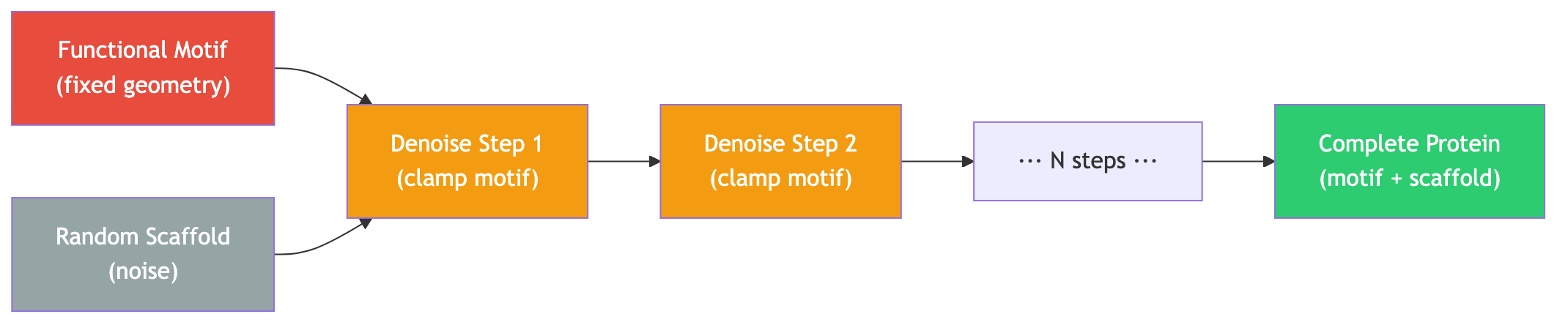
Motif scaffolding. A functional motif — say, a set of catalytic residues arranged in a specific geometry — must be presented by a supporting protein scaffold. RFDiffusion generates the scaffold while holding the motif residues fixed.
Binder design. Given a target protein (for example, a viral surface protein), design a new protein that binds to a specified surface region on the target. This is the key to computational vaccine and therapeutic design.
Symmetric assemblies. Generate proteins with specified symmetry — dimers (\(C_2\)), trimers (\(C_3\)), or higher-order assemblies — that can form cages, rings, or filaments.
Secondary structure conditioning. Specify a desired pattern of helices and sheets, and let the model determine the three-dimensional arrangement.
How Conditioning Works
The simplest and most effective conditioning strategy is inpainting: at each step of the reverse diffusion process, replace the frames at motif positions with the ground-truth values. The model generates the remaining (scaffold) residues conditioned on the fixed motif geometry.
This approach is effective because the denoising network has learned, from thousands of training structures, what kinds of scaffolds are geometrically and energetically plausible. Clamping the motif constrains the solution space to scaffolds that are compatible with the desired functional geometry.
Self-conditioning feeds the model’s own previous prediction back as additional input. During training, with probability 0.5, the model first makes a prediction without self-conditioning, then makes a second prediction that also receives the first prediction as input. This provides the model with a “rough draft” of the final structure, allowing it to make more coherent updates.
Classifier-free guidance provides a continuous knob to control the strength of conditioning. During training, the conditioning signal is randomly dropped. At inference time, the model is run twice — once with conditioning and once without — and the predictions are combined:
\[\hat{x}_0^{\text{guided}} = \hat{x}_0^{\text{uncond}} + s \cdot (\hat{x}_0^{\text{cond}} - \hat{x}_0^{\text{uncond}}),\]where \(s\) is the guidance scale. When \(s = 1\), this reduces to the conditional prediction. When \(s > 1\), the model extrapolates beyond the conditional prediction, producing structures that satisfy the constraints more strongly at the cost of reduced diversity. In practice, guidance scales between 1.0 and 3.0 work well for protein design.
The implementation details of motif conditioning, self-conditioning, and classifier-free guidance are covered in Lecture 10.
5. Experimental Validation and Comparison
Proteins That Actually Work
The ultimate test of any protein design method is experimental validation. RFDiffusion has been validated extensively, with several categories of results reported in the original Nature paper [a]:
Novel folds. RFDiffusion generates backbone topologies never observed in nature. When the corresponding amino acid sequences were designed (using ProteinMPNN [c]), synthesized, and expressed in E. coli, the proteins folded into the predicted structures. Small-angle X-ray scattering (SAXS) and circular dichroism (CD) measurements confirmed the expected size, shape, and secondary structure content.
Symmetric assemblies. By incorporating symmetry constraints (e.g., \(C_3\) for trimers or octahedral symmetry for cages), RFDiffusion designs proteins that self-assemble into multi-subunit architectures. Cryo-electron microscopy confirmed the designed symmetry.
Functional binders. RFDiffusion has designed proteins that bind to therapeutically relevant targets — including influenza hemagglutinin and SARS-CoV-2 receptor binding domain — with nanomolar affinity. This demonstrates the practical potential for drug and vaccine development.
Enzyme scaffolds. By scaffolding around known catalytic motifs (fixing the positions of key catalytic residues), researchers have generated novel enzyme backbones. The model produces scaffolds that hold the catalytic residues in the correct geometry, enabling enzymatic activity.
Comparison with Other Methods
Several groups have developed alternative approaches to protein backbone generation. The following table summarizes the key differences:
| Method | Representation | Symmetry | Generation Approach | Key Advantage |
|---|---|---|---|---|
| RFDiffusion | SE(3) frames | SE(3) equivariant | Diffusion (DDPM) | Pretrained from RoseTTAFold; rich conditioning |
| Chroma | Distance matrix | E(3) invariant | Diffusion | Simpler representation; scalable |
| FrameDiff | SE(3) frames | SE(3) equivariant | Flow matching | Theoretically principled; continuous-time |
| Genie | Backbone angles | None | Autoregressive | Simple; no equivariance overhead |
RFDiffusion’s strength is the combination of SE(3) equivariance, the powerful pretrained RoseTTAFold backbone, and the flexible conditioning mechanisms that enable practical design applications. Chroma trades some geometric expressiveness for a simpler, distance-matrix-based representation. FrameDiff uses the same SE(3) frame representation but replaces the diffusion process with flow matching, which offers cleaner training dynamics. Genie takes the simplest approach, generating backbone angles autoregressively without explicit geometric symmetry.
The field is evolving rapidly, and each method has its niche. But RFDiffusion’s experimental success has established SE(3) diffusion as a dominant paradigm for structure-based protein design.
Key Takeaways
-
Structure determines function. A protein’s three-dimensional backbone geometry directly controls what it can do — from enzyme catalysis to receptor binding to self-assembly. Controlling shape at the angstrom scale means controlling biology.
-
De novo design generates proteins that have never existed in nature. Unlike directed evolution, which optimizes existing proteins, computational design can create entirely new folds, topologies, and functional surfaces.
-
RFDiffusion generates backbones; ProteinMPNN designs sequences. The design pipeline separates the backbone design problem (what shape?) from the sequence design problem (what amino acids?), solving each with a specialized model.
-
Conditional generation makes designs functional. Motif scaffolding holds catalytic residues fixed. Binder design generates complementary surfaces. Symmetric generation produces oligomeric assemblies. Classifier-free guidance controls the conditioning strength.
-
Experimental validation confirms the approach. More than 50% of computationally designed proteins fold as predicted and perform their intended functions — a dramatic improvement over pre-diffusion methods.
-
The companion Lecture 10 covers the SE(3) mathematics. Rotation representations, IGSO(3) noise, equivariant architectures, and the full RFDiffusion training and sampling algorithms are developed there.
References
[a] Watson, J. L., Juergens, D., Bennett, N. R., Trippe, B. L., Yim, J., Eisenach, H. E., ... & Baker, D. (2023). De novo design of protein structure and function with RFdiffusion. Nature, 620(7976), 1089–1100.
[c] Dauparas, J., Anishchenko, I., Bennett, N., Bai, H., Ragotte, R. J., Milles, L. F., ... & Baker, D. (2022). Robust deep learning–based protein sequence design using ProteinMPNN. Science, 378(6615), 49–56.
-
Kuhlman, B., Dantas, G., Ireton, G. C., Varani, G., Stoddard, B. L., & Baker, D. (2003). Design of a novel globular protein fold with atomic-level accuracy. Science, 302(5649), 1364–1368. ↩