AlphaFold: Architecture and Training
This is Lecture 8 of the Protein & Artificial Intelligence course (Spring 2026), co-taught by Prof. Sungsoo Ahn and Prof. Homin Kim at KAIST Graduate School of AI. It is the architecture companion to Lecture 7 (AlphaFold: The Structure Prediction Problem). It assumes familiarity with transformers (Lecture 1) and protein language models (Lectures 5–6). All code examples use PyTorch.
Introduction
Lecture 7 framed the protein structure prediction problem and its significance—from Anfinsen’s hypothesis through CASP14, and from genetic disease to drug discovery. This lecture dissects AlphaFold2’s architecture: the engineering that turned a 50-year challenge into a solved problem. Every major component is examined in turn—input embedding, the Evoformer, the Structure Module, and the FAPE loss—with simplified PyTorch implementations that make the architecture concrete rather than merely conceptual.
Roadmap
| Section | Topic | Why It Is Needed |
|---|---|---|
| 1 | Input embedding | Translates sequences and MSAs into tensor representations |
| 2 | Evoformer | Extracts co-evolutionary and geometric signals |
| 3 | Structure Module | Converts learned features into 3D atomic coordinates |
| 4 | FAPE loss | Defines what “correct structure” means for training |
| 5 | Full pipeline | Assembles the pieces into one coherent system |
| 6 | Computational considerations | Addresses memory, speed, and scaling |
1. Input Embedding: Translating Biology into Tensors
Every deep learning system must bridge the gap between its domain and the world of tensors. For AlphaFold2, this means encoding amino acid sequences, evolutionary alignments, and (optionally) structural templates into numerical representations.
1.1 What Goes In
AlphaFold2 accepts three categories of input:
Target sequence. The protein whose structure we want to predict, represented as a string of amino acid identifiers. A sequence like MVLSPADKTN... is converted to numerical indices (methionine \(\to\) 0, valine \(\to\) 1, and so on) and then to one-hot vectors of length 21 (20 standard amino acids plus a gap token).
Multiple sequence alignment. Thousands of related sequences, each aligned to the target. Each position in each sequence is encoded with features indicating amino acid identity, insertion counts, and deletion states—49 features per position in total.
Template structures1 (optional). Experimentally determined structures of related proteins. If the database contains a homolog with, say, 40% sequence identity, its backbone coordinates provide geometric clues.
1.2 Creating the Initial Representations
The embedding layer transforms raw inputs into the MSA and pair representations that the Evoformer will refine. The pair representation starts simple: an additive combination of left-residue features, right-residue features, and relative-position encodings.
import torch
import torch.nn as nn

class InputEmbedding(nn.Module):
    """Embed input features into MSA and pair representations.

    Dimensions:
        c_m: MSA representation feature size (default 256)
        c_z: pair representation feature size (default 128)
    """

    def __init__(self, c_m: int = 256, c_z: int = 128):
        super().__init__()
        self.c_m = c_m
        self.c_z = c_z

        # Project 49-dim MSA features to c_m
        self.msa_embedding = nn.Linear(49, c_m)

        # Separate projections for left / right residues in the pair
        self.left_single = nn.Linear(21, c_z)
        self.right_single = nn.Linear(21, c_z)

        # Relative position: clipped to [-32, +32], giving 65 bins
        self.relpos_embedding = nn.Embedding(65, c_z)

    def forward(self, msa_feat, target_feat, residue_index):
        """
        Args:
            msa_feat:      [N_seq, L, 49]  per-sequence, per-position features
            target_feat:   [L, 21]          one-hot target sequence
            residue_index: [L]              integer residue positions

        Returns:
            msa_repr:  [N_seq, L, c_m]
            pair_repr: [L, L, c_z]
        """
        # --- MSA representation ---
        msa_repr = self.msa_embedding(msa_feat)  # [N_seq, L, c_m]

        # --- Pair representation ---
        left  = self.left_single(target_feat)     # [L, c_z]
        right = self.right_single(target_feat)    # [L, c_z]
        pair_repr = left[:, None, :] + right[None, :, :]  # broadcast to [L, L, c_z]

        # Add relative position encoding
        d = residue_index[:, None] - residue_index[None, :]   # [L, L]
        d = torch.clamp(d + 32, 0, 64)  # shift so range is [0, 64]
        pair_repr = pair_repr + self.relpos_embedding(d)

        return msa_repr, pair_repr
The relative position encoding gives the network a prior: residues that are close in sequence (like positions 15 and 16) receive different encodings than residues far apart (like positions 15 and 150). This prior is biologically sensible because sequence-local residues are more likely to be spatially close.
1.3 Key Dimensions
Several dimension constants appear throughout AlphaFold2. Keeping track of them helps when reading code or the original paper.
| Representation | Shape | Typical size | Description |
|---|---|---|---|
| MSA | \([N_{\text{seq}} \times L \times c_m]\) | \(c_m = 256\) | Per-sequence, per-residue features |
| Pair | \([L \times L \times c_z]\) | \(c_z = 128\) | Pairwise residue relationships |
| Single | \([L \times c_s]\) | \(c_s = 384\) | Per-residue features for Structure Module |
2. The Evoformer: Where Evolution Meets Attention
The Evoformer is the heart of AlphaFold2. It is a stack of 48 nearly identical blocks, each of which refines both the MSA representation and the pair representation.

The name telegraphs its purpose: a transformer designed to process evolutionary information.
What makes the Evoformer distinctive is not raw size but architectural specificity. Every sub-component targets a particular biological signal. We examine each in turn.
2.1 MSA Row Attention with Pair Bias
What it does. Within a single sequence of the MSA, each position attends to every other position. This is analogous to self-attention in a standard transformer, but with an important addition: the attention logits are biased by the pair representation.
Why it matters. When position \(i\) decides how much attention to pay to position \(j\), it considers not only the MSA features at those positions but also what the pair representation says about the \((i, j)\) relationship. If the pair representation encodes that positions \(i\) and \(j\) are likely in structural contact, the attention mechanism gives them more opportunity to exchange information.
This creates a feedback loop. The pair representation influences how the MSA is processed, and later, information from the MSA will update the pair representation.
Formally, given query \(Q\), key \(K\), and value \(V\) matrices derived from the MSA representation, and a bias term \(b_{ij}\) derived from the pair representation:
\[\text{Attention}(Q, K, V) = \text{softmax}\!\left(\frac{QK^\top}{\sqrt{d_k}} + b_{ij}\right) V\]where \(d_k\) is the dimension of each attention head.
class MSARowAttentionWithPairBias(nn.Module):
    """MSA row-wise self-attention, biased by the pair representation.

    For each sequence s in the MSA, positions attend to each other
    along the residue axis. The pair representation injects relational
    information into the attention logits.
    """

    def __init__(self, c_m: int = 256, c_z: int = 128, n_heads: int = 8):
        super().__init__()
        self.c_m = c_m
        self.n_heads = n_heads
        self.head_dim = c_m // n_heads

        self.layer_norm_m = nn.LayerNorm(c_m)
        self.layer_norm_z = nn.LayerNorm(c_z)

        # Standard Q / K / V projections
        self.to_q = nn.Linear(c_m, c_m, bias=False)
        self.to_k = nn.Linear(c_m, c_m, bias=False)
        self.to_v = nn.Linear(c_m, c_m, bias=False)

        # Project pair features to per-head bias scalars
        self.pair_bias = nn.Linear(c_z, n_heads, bias=False)

        # Gated output projection
        self.to_out = nn.Linear(c_m, c_m)
        self.gate   = nn.Linear(c_m, c_m)

    def forward(self, msa_repr, pair_repr):
        """
        Args:
            msa_repr:  [N_seq, L, c_m]
            pair_repr: [L, L, c_z]
        Returns:
            updated msa_repr: [N_seq, L, c_m]
        """
        N_seq, L, _ = msa_repr.shape

        m = self.layer_norm_m(msa_repr)
        z = self.layer_norm_z(pair_repr)

        # Q, K, V  ->  [N_seq, L, n_heads, head_dim]
        q = self.to_q(m).view(N_seq, L, self.n_heads, self.head_dim)
        k = self.to_k(m).view(N_seq, L, self.n_heads, self.head_dim)
        v = self.to_v(m).view(N_seq, L, self.n_heads, self.head_dim)

        # Attention logits: [N_seq, n_heads, L, L]
        attn = torch.einsum('bihd,bjhd->bhij', q, k) / (self.head_dim ** 0.5)

        # Pair bias: [L, L, n_heads] -> [1, n_heads, L, L]
        bias = self.pair_bias(z).permute(2, 0, 1).unsqueeze(0)
        attn = attn + bias

        attn = torch.softmax(attn, dim=-1)
        out  = torch.einsum('bhij,bjhd->bihd', attn, v)
        out  = out.reshape(N_seq, L, self.c_m)

        # Gating: the network learns when to incorporate new information
        gate = torch.sigmoid(self.gate(m))
        out  = gate * self.to_out(out)

        return msa_repr + out  # residual connection
The gating mechanism at the output deserves attention. Rather than always adding the full attention output, the network learns a per-element sigmoid gate that controls how much new information to incorporate. This pattern appears throughout AlphaFold2 and helps stabilize gradient flow during training.
2.2 MSA Column Attention
What it does. While row attention examines relationships within a single sequence, column attention looks at the same position across different sequences in the MSA.
Why it matters. Column attention is where co-evolutionary signals become explicit. When the network attends across sequences at a given column, it discovers patterns such as “whenever this position is hydrophobic, that other position (in the same column of the pair representation) also tends to be hydrophobic.” Each sequence in the MSA represents a different evolutionary experiment—a different organism’s solution to the same folding problem. Column attention aggregates the lessons of those experiments.
This operation is computationally expensive because it attends over potentially thousands of sequences. AlphaFold2 mitigates this cost by sampling down to 512 sequences for the extra MSA stack and by using axial attention: row and column attention are applied sequentially rather than computing full two-dimensional attention over the entire \(N_{\text{seq}} \times L\) grid2.
2.3 Triangular Updates: Enforcing Geometric Consistency
Now we come to one of AlphaFold2’s most elegant ideas.
Consider three residues \(A\), \(B\), and \(C\). If \(A\) is close to \(B\) and \(B\) is close to \(C\), what can we infer about the \(A\)–\(C\) relationship? In principle, \(A\) and \(C\) could be anywhere within the sum of the two distances (the triangle inequality). But proteins are densely packed, and real constraints are far tighter than the worst-case triangle inequality.
The triangular updates pass messages around triangles in the pair representation, enforcing this kind of three-body consistency.
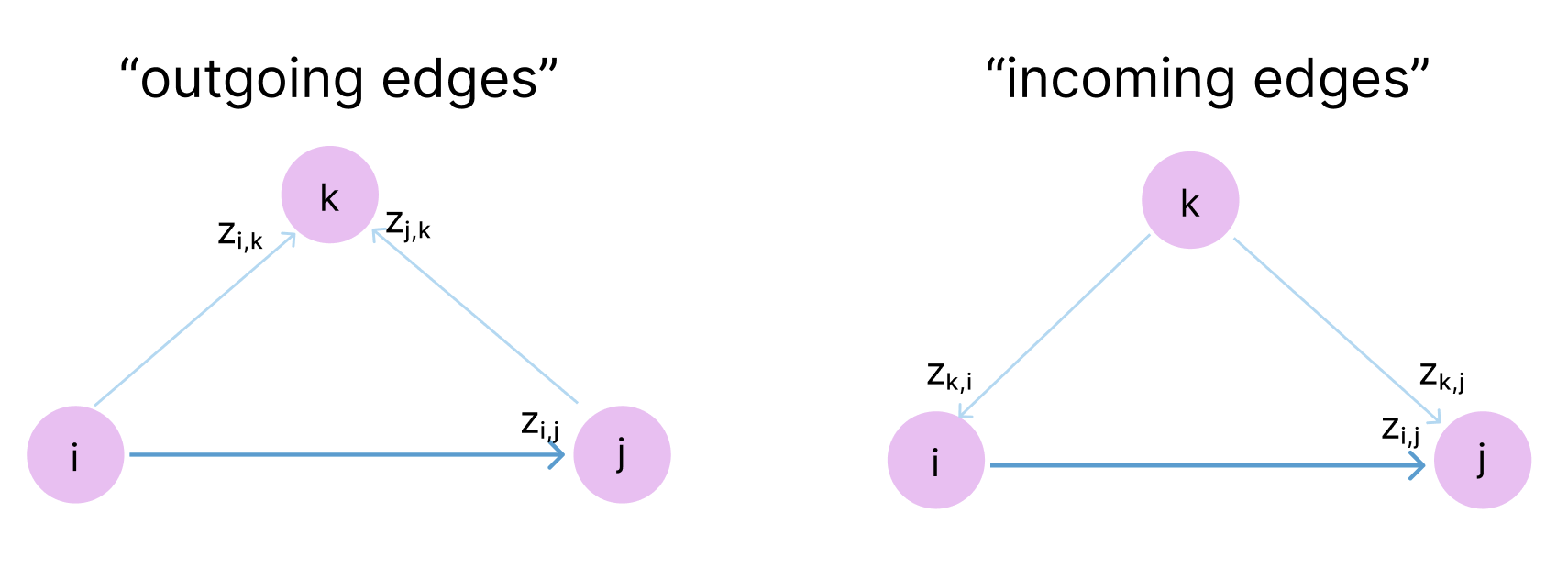
There are four triangular operations in each Evoformer block—two multiplicative updates and two attention variants—each providing a different view of the geometric constraints.
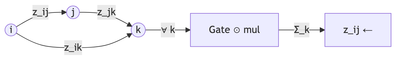
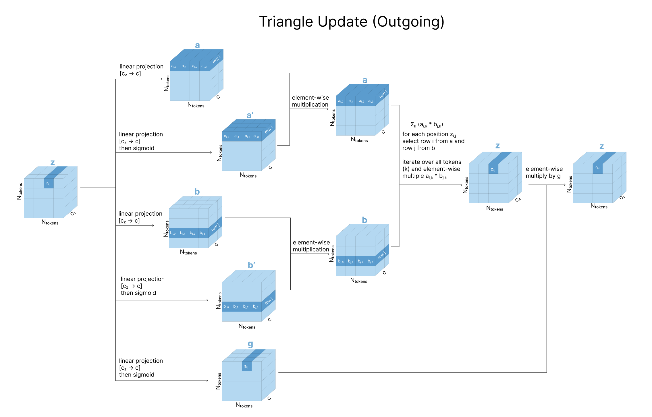
2.3.1 Triangular Multiplicative Update (Outgoing Edges)
For each pair \((i, j)\), aggregate information from all pairs \((i, k)\) and \((j, k)\) that share a third node \(k\):
\[z_{ij} \leftarrow z_{ij} + \sum_k a_{ik} \odot b_{jk}\]Here \(a_{ik}\) and \(b_{jk}\) are gated linear projections of the pair representation, and \(\odot\) denotes element-wise multiplication. The sum over \(k\) accumulates evidence from every possible third vertex.
2.3.2 Triangular Multiplicative Update (Incoming Edges)
The same idea, but the summation runs over the other index:
\[z_{ij} \leftarrow z_{ij} + \sum_k a_{ki} \odot b_{kj}\]The outgoing variant asks “which residues do \(i\) and \(j\) both point to?” The incoming variant asks “which residues both point to \(i\) and \(j\)?”
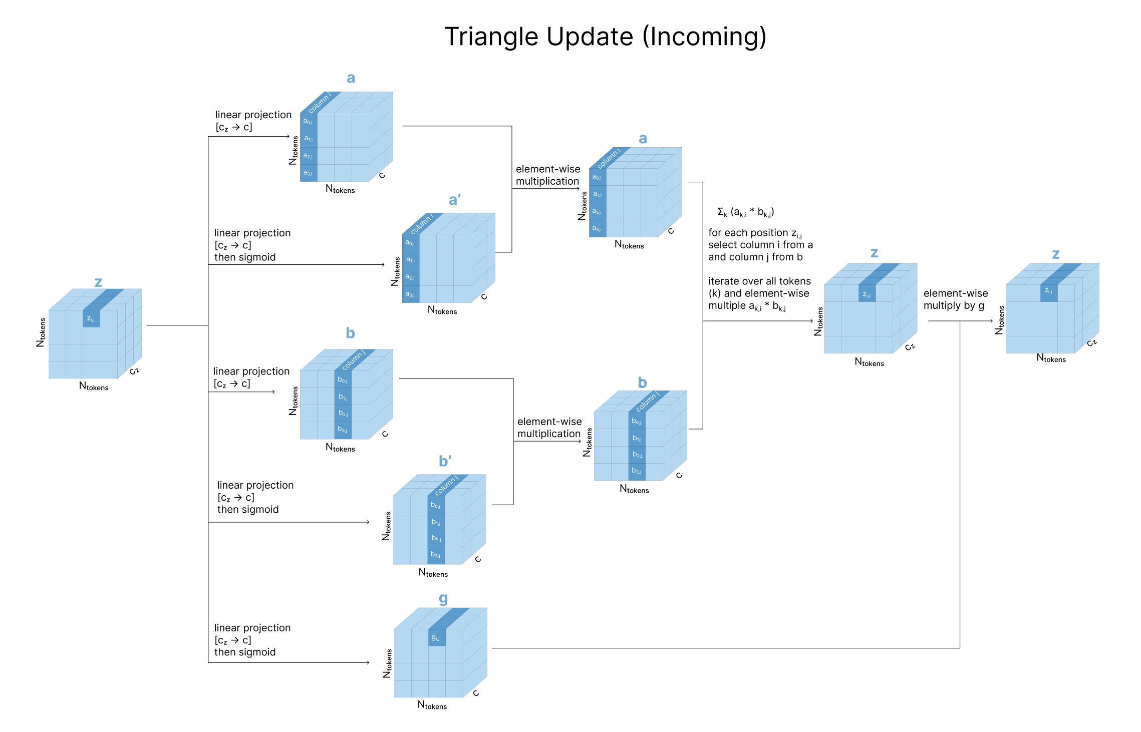
class TriangularMultiplicativeUpdate(nn.Module):
    """Triangular multiplicative update for the pair representation.

    Enforces three-body geometric consistency by aggregating
    information from triangles (i, j, k) in the pair graph.

    Args:
        c_z:      pair representation feature dimension
        c_hidden: hidden projection dimension
        mode:     'outgoing' or 'incoming'
    """

    def __init__(self, c_z: int = 128, c_hidden: int = 128, mode: str = 'outgoing'):
        super().__init__()
        self.mode = mode
        self.layer_norm = nn.LayerNorm(c_z)

        # Gated projections for the two edges of each triangle
        self.left_proj  = nn.Linear(c_z, c_hidden)
        self.right_proj = nn.Linear(c_z, c_hidden)
        self.left_gate  = nn.Linear(c_z, c_hidden)
        self.right_gate = nn.Linear(c_z, c_hidden)

        # Output with gating
        self.output_gate = nn.Linear(c_z, c_z)
        self.output_proj = nn.Linear(c_hidden, c_z)
        self.final_norm  = nn.LayerNorm(c_hidden)

    def forward(self, pair_repr):
        """
        Args:
            pair_repr: [L, L, c_z]
        Returns:
            updated pair_repr: [L, L, c_z]
        """
        z = self.layer_norm(pair_repr)

        # Project and gate each edge
        left  = self.left_proj(z)  * torch.sigmoid(self.left_gate(z))
        right = self.right_proj(z) * torch.sigmoid(self.right_gate(z))

        if self.mode == 'outgoing':
            # z_ij += sum_k  left[i,k] * right[j,k]
            out = torch.einsum('ikc,jkc->ijc', left, right)
        else:
            # z_ij += sum_k  left[k,i] * right[k,j]
            out = torch.einsum('kic,kjc->ijc', left, right)

        out  = self.final_norm(out)
        out  = self.output_proj(out)
        gate = torch.sigmoid(self.output_gate(pair_repr))

        return pair_repr + gate * out
2.3.3 Triangular Attention
The triangular attention operations serve a similar purpose but use attention rather than element-wise multiplication to aggregate information. Two variants exist—starting-node and ending-node—providing complementary views of the triangle.
class TriangularAttention(nn.Module):
    """Triangular self-attention over the pair representation.

    For 'starting' mode: for each starting node i, pairs (i,j) attend
    over other pairs (i,k), biased by (j,k).
    For 'ending' mode: transpose, attend, transpose back.
    """

    def __init__(self, c_z: int = 128, n_heads: int = 4, mode: str = 'starting'):
        super().__init__()
        self.c_z = c_z
        self.n_heads = n_heads
        self.head_dim = c_z // n_heads
        self.mode = mode

        self.layer_norm = nn.LayerNorm(c_z)
        self.to_q = nn.Linear(c_z, c_z, bias=False)
        self.to_k = nn.Linear(c_z, c_z, bias=False)
        self.to_v = nn.Linear(c_z, c_z, bias=False)

        # Bias derived from the pair representation itself
        self.bias_proj = nn.Linear(c_z, n_heads, bias=False)

        self.to_out = nn.Linear(c_z, c_z)
        self.gate   = nn.Linear(c_z, c_z)

    def forward(self, pair_repr):
        """
        Args:
            pair_repr: [L, L, c_z]
        Returns:
            updated pair_repr: [L, L, c_z]
        """
        L = pair_repr.shape[0]

        if self.mode == 'ending':
            pair_repr = pair_repr.transpose(0, 1)

        z = self.layer_norm(pair_repr)

        q = self.to_q(z).view(L, L, self.n_heads, self.head_dim)
        k = self.to_k(z).view(L, L, self.n_heads, self.head_dim)
        v = self.to_v(z).view(L, L, self.n_heads, self.head_dim)

        # For each row i, positions j attend over positions k
        attn = torch.einsum('ijhd,ikhd->hijk', q, k) / (self.head_dim ** 0.5)

        # Bias from pair representation
        bias = self.bias_proj(z).permute(2, 0, 1).unsqueeze(1)
        attn = attn + bias

        attn = torch.softmax(attn, dim=-1)
        out  = torch.einsum('hijk,ikhd->ijhd', attn, v)
        out  = out.reshape(L, L, self.c_z)

        gate   = torch.sigmoid(self.gate(pair_repr))
        out    = gate * self.to_out(out)
        result = pair_repr + out

        if self.mode == 'ending':
            result = result.transpose(0, 1)

        return result
Why both multiplicative updates and attention? They capture different aspects of geometric constraints. The multiplicative updates are “hard” operations that directly compute products summed over triangle vertices. The attention operations are “soft,” letting the network learn which triangles matter most for each pair. Together they provide complementary pathways for enforcing geometric consistency.
2.4 Outer Product Mean: Bridging MSA and Pairs
The MSA representation and pair representation need to communicate. The outer product mean is the primary pathway from MSA to pairs.
The intuition is straightforward. If two positions have correlated feature patterns across the MSA, they are probably structurally related. The outer product computes exactly this correlation:
\[z_{ij} \leftarrow z_{ij} + \frac{1}{N_{\text{seq}}} \sum_{s=1}^{N_{\text{seq}}} m_{si} \otimes m_{sj}\]where \(m_{si}\) is the MSA feature vector for sequence \(s\) at position \(i\), and \(\otimes\) denotes the outer product. For each pair \((i, j)\), we compute the outer product of the projected MSA features at positions \(i\) and \(j\), then average over all sequences.
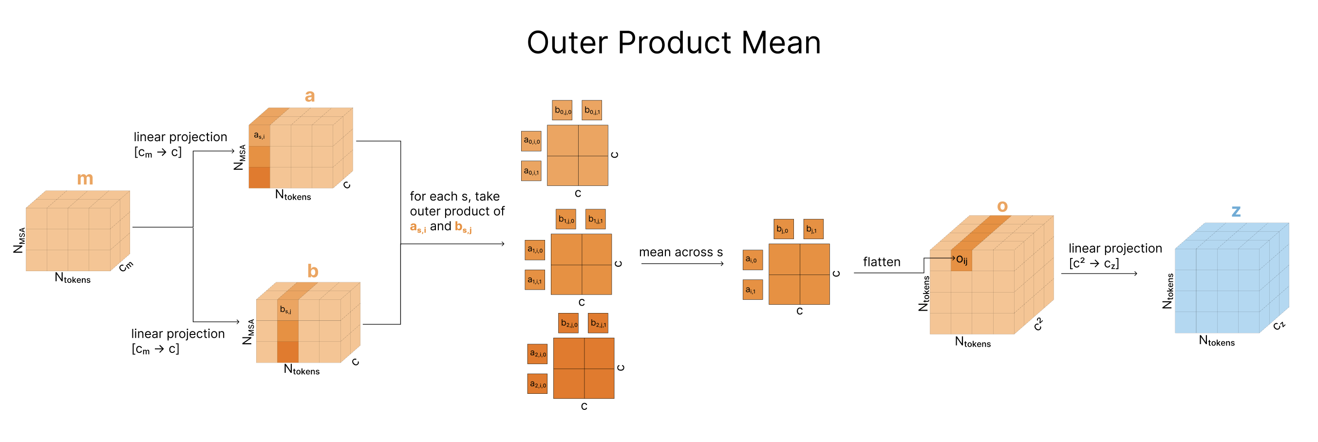
class OuterProductMean(nn.Module):
    """Transfer information from the MSA to the pair representation
    via the mean of outer products across sequences.

    This is the primary MSA -> pair communication channel.
    """

    def __init__(self, c_m: int = 256, c_z: int = 128, c_hidden: int = 32):
        super().__init__()
        self.layer_norm  = nn.LayerNorm(c_m)
        self.left_proj   = nn.Linear(c_m, c_hidden)
        self.right_proj  = nn.Linear(c_m, c_hidden)
        self.output      = nn.Linear(c_hidden * c_hidden, c_z)

    def forward(self, msa_repr):
        """
        Args:
            msa_repr: [N_seq, L, c_m]
        Returns:
            pair_update: [L, L, c_z]
        """
        m = self.layer_norm(msa_repr)

        left  = self.left_proj(m)    # [N_seq, L, c_hidden]
        right = self.right_proj(m)   # [N_seq, L, c_hidden]

        # Outer product, averaged over sequences
        outer = torch.einsum('sic,sjd->ijcd', left, right)
        outer = outer / msa_repr.shape[0]

        # Flatten the outer-product dimensions and project
        outer = outer.reshape(outer.shape[0], outer.shape[1], -1)
        return self.output(outer)
2.5 The Complete Evoformer Block
Each Evoformer block orchestrates all the components described above. The information flow within a single block is as follows:
+-------------------------------------------------------------+
|                      Evoformer Block                         |
+-------------------------------------------------------------+
|                                                              |
|  MSA Stack:                    Pair Stack:                   |
|  +--------------------+       +------------------------+    |
|  | MSA Row Attention  |       | Triangular Mult. Update|    |
|  | (with pair bias)   |       | (outgoing edges)       |    |
|  +--------------------+       +------------------------+    |
|           |                            |                     |
|           v                            v                     |
|  +--------------------+       +------------------------+    |
|  | MSA Column         |       | Triangular Mult. Update|    |
|  | Attention           |       | (incoming edges)       |    |
|  +--------------------+       +------------------------+    |
|           |                            |                     |
|           v                            v                     |
|  +--------------------+       +------------------------+    |
|  | MSA Transition     |       | Triangular Attention   |    |
|  | (feed-forward)     |       | (starting node)        |    |
|  +--------------------+       +------------------------+    |
|           |                            |                     |
|           |                            v                     |
|           |               +------------------------+        |
|           |               | Triangular Attention   |        |
|           |               | (ending node)          |        |
|           |               +------------------------+        |
|           |                            |                     |
|           |                            v                     |
|           |               +------------------------+        |
|           |               | Pair Transition        |        |
|           |               | (feed-forward)         |        |
|           |               +------------------------+        |
|           |                            |                     |
|           v                            v                     |
|  +--------------------------------------------+             |
|  |         Outer Product Mean (MSA -> Pair)    |             |
|  +--------------------------------------------+             |
|                                                              |
+-------------------------------------------------------------+
After 48 of these blocks, the MSA representation has been refined through thousands of attention operations, and the pair representation encodes detailed spatial relationships between all residue pairs. The pair representation now functions as a predicted distance map—a blurry but informative picture of which residues are close in three-dimensional space.
But a distance map is not yet a structure. The next step converts pairwise relationships into actual atomic coordinates.
3. The Structure Module: From Features to Coordinates
The Structure Module is where AlphaFold2 produces its final output: three-dimensional atomic coordinates for every residue. This component introduces Invariant Point Attention (IPA), arguably the most important architectural innovation in the system.
3.1 The Challenge of Three-Dimensional Structure
Protein structures exist in three-dimensional Euclidean space, and that space has symmetries. If you rotate a protein by 90 degrees, it is still the same protein. If you translate it 10 angstroms to the left, the structure is unchanged. These symmetries form the group \(SE(3)\)—the special Euclidean group in three dimensions, consisting of all rotations and translations3.
Any valid structure prediction method must respect these symmetries. Earlier approaches sidestepped the issue by predicting distance matrices or contact maps, which are naturally rotation- and translation-invariant. AlphaFold2 wanted to predict actual coordinates, which required building invariance directly into the architecture.
3.2 Frames: A Language for Protein Geometry
AlphaFold2’s solution is to represent each residue as a rigid body frame—a local coordinate system defined by a rotation and a translation. The backbone atoms of each residue (N, C\(_\alpha\), C) define a natural reference frame.
A frame \(T_i = (R_i, \vec{t}_i)\) for residue \(i\) consists of:
- \(R_i \in SO(3)\): a \(3 \times 3\) rotation matrix (orthogonal, determinant 1)
- \(\vec{t}_i \in \mathbb{R}^3\): a translation vector (the position of C\(_\alpha\))
Any point in space can be expressed either in global coordinates or in the local coordinate system of any frame. Converting between these viewpoints is fundamental to how the Structure Module operates.
class Rigid:
    """Rigid body transformation: rotation + translation.

    Represents a frame T = (R, t) that maps local coordinates
    to global coordinates via  x_global = R @ x_local + t.
    """

    def __init__(self, rots, trans):
        """
        Args:
            rots:  [*, 3, 3] rotation matrices
            trans: [*, 3]    translation vectors
        """
        self.rots  = rots
        self.trans = trans

    @staticmethod
    def identity(shape, device='cpu'):
        """Create identity frames (no rotation, no translation)."""
        rots  = torch.eye(3, device=device).expand(*shape, 3, 3).clone()
        trans = torch.zeros(*shape, 3, device=device)
        return Rigid(rots, trans)

    def compose(self, other):
        """Compose two rigid transformations: self * other.

        If self = (R1, t1) and other = (R2, t2), then
        composed = (R1 @ R2, R1 @ t2 + t1).
        """
        new_rots  = torch.einsum('...ij,...jk->...ik', self.rots, other.rots)
        new_trans = (torch.einsum('...ij,...j->...i', self.rots, other.trans)
                     + self.trans)
        return Rigid(new_rots, new_trans)

    def apply(self, points):
        """Apply transformation to points: R @ x + t."""
        return torch.einsum('...ij,...j->...i', self.rots, points) + self.trans

    def invert(self):
        """Compute the inverse transformation: (R^T, -R^T @ t)."""
        inv_rots  = self.rots.transpose(-1, -2)
        inv_trans = -torch.einsum('...ij,...j->...i', inv_rots, self.trans)
        return Rigid(inv_rots, inv_trans)
3.3 Invariant Point Attention (IPA)
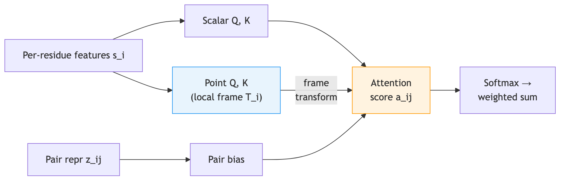
Invariant Point Attention is the mechanism that lets the network reason about three-dimensional geometry while remaining invariant to global rotations and translations.
Standard attention computes similarity between queries and keys, both of which are learned projections of input features. IPA extends this by introducing point queries and point keys—three-dimensional coordinates expressed in each residue’s local frame.
When residue \(i\) attends to residue \(j\), the attention score combines three components:
- Scalar attention. Standard query-key dot product on feature vectors, identical to a regular transformer head.
- Pair bias. A projection of the pair representation entry \((i, j)\), injecting relational information.
- Point attention. The squared Euclidean distance between query points and key points when both are expressed in a common reference frame.
The key to invariance is component 3. Each residue generates query points \(\vec{q}_{ip}\) and key points \(\vec{k}_{jp}\) in its own local coordinate system (the subscript \(p\) indexes over multiple query/key points per head). To compare them, we transform residue \(j\)’s key points into residue \(i\)’s coordinate frame by applying \(T_i^{-1} \circ T_j\). The squared distance between the transformed key points and the query points contributes to the attention logit:
\[a_{ij} = \underbrace{q_i \cdot k_j}_{\text{scalar}} + \underbrace{b_{ij}}_{\text{pair bias}} - \underbrace{\frac{w_c}{2} \sum_p \lvert T_i^{-1}(T_j(\vec{k}_{jp})) - \vec{q}_{ip} \rvert^2}_{\text{point distance}}\]where \(w_c\) is a learnable per-head weight that controls how strongly spatial proximity influences attention. The negative sign ensures that closer points receive higher attention.
This distance is invariant to global rotations and translations because both sets of points are expressed relative to the same local frame.
class InvariantPointAttention(nn.Module):
    """Invariant Point Attention (IPA).

    SE(3)-invariant attention that combines scalar features,
    pair features, and 3D point features expressed in local frames.

    Args:
        c_s:         single representation dimension
        c_z:         pair representation dimension
        n_heads:     number of attention heads
        n_qk_points: number of query/key point vectors per head
        n_v_points:  number of value point vectors per head
    """

    def __init__(self, c_s=384, c_z=128, n_heads=12,
                 n_qk_points=4, n_v_points=8):
        super().__init__()
        self.c_s = c_s
        self.n_heads = n_heads
        self.head_dim = c_s // n_heads
        self.n_qk_points = n_qk_points
        self.n_v_points  = n_v_points

        # Scalar Q / K / V
        self.to_q = nn.Linear(c_s, c_s, bias=False)
        self.to_k = nn.Linear(c_s, c_s, bias=False)
        self.to_v = nn.Linear(c_s, c_s, bias=False)

        # Point Q / K / V  (3D coordinates in local frame)
        self.to_q_points = nn.Linear(c_s, n_heads * n_qk_points * 3)
        self.to_k_points = nn.Linear(c_s, n_heads * n_qk_points * 3)
        self.to_v_points = nn.Linear(c_s, n_heads * n_v_points  * 3)

        # Pair bias
        self.pair_bias = nn.Linear(c_z, n_heads, bias=False)

        # Learnable per-head weight for the point-distance term
        self.head_weights = nn.Parameter(torch.zeros(n_heads))

        # Output projection (scalar + point + pair outputs concatenated)
        out_dim = c_s + n_heads * n_v_points * 3 + n_heads * c_z
        self.to_out = nn.Linear(out_dim, c_s)

    def forward(self, single_repr, pair_repr, rigids):
        """
        Args:
            single_repr: [L, c_s]   per-residue features
            pair_repr:   [L, L, c_z] pairwise features
            rigids:      Rigid with [L] frames
        Returns:
            updated single_repr: [L, c_s]
        """
        L = single_repr.shape[0]

        # --- Scalar branch ---
        q = self.to_q(single_repr).view(L, self.n_heads, self.head_dim)
        k = self.to_k(single_repr).view(L, self.n_heads, self.head_dim)
        v = self.to_v(single_repr).view(L, self.n_heads, self.head_dim)

        # --- Point branch ---
        q_pts = self.to_q_points(single_repr).view(
            L, self.n_heads, self.n_qk_points, 3)
        k_pts = self.to_k_points(single_repr).view(
            L, self.n_heads, self.n_qk_points, 3)
        v_pts = self.to_v_points(single_repr).view(
            L, self.n_heads, self.n_v_points, 3)

        # Transform points from local frames to global frame
        q_pts_global = rigids.apply(
            q_pts.reshape(L, -1, 3)).view(L, self.n_heads, self.n_qk_points, 3)
        k_pts_global = rigids.apply(
            k_pts.reshape(L, -1, 3)).view(L, self.n_heads, self.n_qk_points, 3)
        v_pts_global = rigids.apply(
            v_pts.reshape(L, -1, 3)).view(L, self.n_heads, self.n_v_points, 3)

        # --- Attention logits ---
        # 1. Scalar attention
        attn_scalar = torch.einsum('ihd,jhd->hij', q, k) / (self.head_dim ** 0.5)

        # 2. Point attention (negative squared distance -> closer = higher)
        pt_diff    = (q_pts_global[:, None, :, :, :]
                      - k_pts_global[None, :, :, :, :])        # [L, L, H, P, 3]
        pt_dist_sq = (pt_diff ** 2).sum(dim=-1).sum(dim=-1)    # [L, L, H]
        w_c        = torch.softplus(self.head_weights)
        attn_pts   = -0.5 * w_c * pt_dist_sq.permute(2, 0, 1) # [H, L, L]

        # 3. Pair bias
        attn_pair = self.pair_bias(pair_repr).permute(2, 0, 1)  # [H, L, L]

        # Combine and softmax
        attn = attn_scalar.permute(2, 0, 1) + attn_pts + attn_pair
        attn = torch.softmax(attn, dim=-1)  # [H, L, L]

        # --- Attended values ---
        # Scalar output
        out_scalar = torch.einsum('hij,jhd->ihd', attn, v).reshape(L, self.c_s)

        # Point output (global frame -> local frame)
        out_pts_global = torch.einsum('hij,jhpc->ihpc', attn, v_pts_global)
        out_pts_local  = rigids.invert().apply(
            out_pts_global.reshape(L, -1, 3))
        out_pts = out_pts_local.reshape(L, -1)

        # Pair output
        out_pair = torch.einsum('hij,ijc->ihc', attn, pair_repr).reshape(L, -1)

        # Concatenate all outputs and project
        out = torch.cat([out_scalar, out_pts, out_pair], dim=-1)
        return self.to_out(out)
3.4 Iterative Refinement
The Structure Module does not predict coordinates in a single pass. Instead, it initializes all residue frames to the identity transformation—placing every residue at the origin with default orientation—and iteratively refines them through 8 layers of IPA.
Each iteration:
- Applies IPA to update per-residue features, using the current frames.
- Passes features through a transition (feed-forward) network.
- Predicts a small update to each residue’s frame (a rotation and translation).
- Composes this update with the current frame.
This iterative approach resembles message passing in a graph neural network. Early iterations establish coarse global topology (“this helix packs against that sheet”). Later iterations fine-tune local geometry (“this side chain points inward, not outward”).
class StructureModule(nn.Module):
    """Structure Module: iteratively refines residue frames
    from identity to the predicted 3D structure.

    Takes the refined MSA and pair representations from the
    Evoformer and produces C-alpha coordinates.

    Args:
        c_s:      single representation dimension
        c_z:      pair representation dimension
        n_layers: number of IPA refinement iterations
    """

    def __init__(self, c_s: int = 384, c_z: int = 128, n_layers: int = 8):
        super().__init__()
        self.input_proj = nn.Linear(256, c_s)  # project c_m -> c_s

        self.ipa_layers = nn.ModuleList([
            InvariantPointAttention(c_s, c_z) for _ in range(n_layers)
        ])

        self.transitions = nn.ModuleList([
            nn.Sequential(
                nn.LayerNorm(c_s),
                nn.Linear(c_s, c_s * 4),
                nn.ReLU(),
                nn.Linear(c_s * 4, c_s),
            ) for _ in range(n_layers)
        ])

        # Predict 6-DOF frame update: 3 rotation angles + 3 translation
        self.backbone_update = nn.Linear(c_s, 6)

    def forward(self, msa_repr, pair_repr):
        """
        Args:
            msa_repr:  [N_seq, L, c_m]
            pair_repr: [L, L, c_z]
        Returns:
            coords: [L, 3]  predicted C-alpha coordinates
            frames: Rigid    per-residue frames
        """
        L = pair_repr.shape[0]

        # Initialize single representation from first row of the MSA
        # (the first row is the target sequence)
        single = self.input_proj(msa_repr[0])  # [L, c_s]

        # All frames start at identity
        frames = Rigid.identity((L,), device=single.device)

        for ipa, transition in zip(self.ipa_layers, self.transitions):
            # 1. IPA: update single representation using current frames
            single = single + ipa(single, pair_repr, frames)

            # 2. Transition: per-residue feed-forward
            single = single + transition(single)

            # 3. Predict frame update (small rotation + translation)
            update = self.backbone_update(single)
            rot_angles   = update[:, :3] * 0.1   # scale down for stability
            trans_update = update[:, 3:]

            # Simplified: identity rotation + translation
            # (full implementation uses quaternion parameterization)
            rot_mat = torch.eye(3, device=single.device).unsqueeze(0).expand(
                L, -1, -1).clone()
            frame_update = Rigid(rot_mat, trans_update)

            # 4. Compose update with current frames
            frames = frames.compose(frame_update)

        # C-alpha coordinates are the origins of the final frames
        coords = frames.trans
        return coords, frames
A note on the rotation parameterization: the code above uses a simplified identity rotation for clarity. The actual AlphaFold2 implementation parameterizes rotations using quaternions, which avoid gimbal lock and compose correctly under small updates4.
4. FAPE Loss: Teaching Geometry Through Local Frames
With the architecture in place, we turn to the question of how AlphaFold2 learns. This requires a loss function that captures what it means for a predicted structure to be correct.
4.1 The Problem with RMSD
The standard metric for comparing protein structures is root-mean-square deviation (RMSD): optimally superimpose the predicted and true structures, then compute the average squared displacement of corresponding atoms. RMSD has been the workhorse of structural biology for decades, but it has several problems as a training loss:
- Optimal superposition is not cleanly differentiable. Finding the rotation that minimizes the error involves an eigenvalue decomposition5 (the Kabsch algorithm), which complicates gradient computation.
- RMSD treats all errors equally. A 2-angstrom error in a floppy loop is penalized the same as a 2-angstrom error in a rigid beta sheet, even though the loop error might be physically reasonable.
- Global sensitivity. A single badly predicted domain can dominate the RMSD, masking accurate predictions elsewhere.
4.2 Frame Aligned Point Error (FAPE)
AlphaFold2’s answer is Frame Aligned Point Error (FAPE). Instead of measuring error in global coordinates, FAPE measures error in local coordinate frames.
For each residue \(i\) with its local frame \(T_i\), we express the positions of all other residues \(j\) in that frame. We do this for both the predicted structure and the true structure. The FAPE loss is the average discrepancy:
\[\text{FAPE} = \frac{1}{L^2} \sum_{i=1}^{L} \sum_{j=1}^{L} \left\lvert T_i^{\text{true},-1}(\vec{x}_j^{\text{true}}) - T_i^{\text{pred},-1}(\vec{x}_j^{\text{pred}}) \right\rvert\]Why is this a good loss function?
- SE(3) invariance. Global rotations and translations cancel out because everything is measured relative to local frames.
- Local accuracy emphasis. If a flexible loop is locally correct but globally displaced, errors in one part of the loop do not propagate to inflate the loss at distant residues.
- Dense gradient signal. Every pair \((i, j)\) contributes independently, providing \(L^2\) terms of supervision rather than a single global scalar.
def fape_loss(pred_frames, pred_coords, true_frames, true_coords,
              clamp_distance=10.0):
    """Frame Aligned Point Error (FAPE) loss.

    Measures structural accuracy in local coordinate frames,
    providing SE(3)-invariant supervision.

    Args:
        pred_frames:    Rigid with [L] predicted frames
        pred_coords:    [L, 3] predicted C-alpha positions
        true_frames:    Rigid with [L] ground-truth frames
        true_coords:    [L, 3] ground-truth C-alpha positions
        clamp_distance: maximum per-pair error (angstroms)

    Returns:
        loss: scalar FAPE loss
    """
    L = pred_coords.shape[0]

    # Express all coordinates in each frame's local system
    # pred_local[i, j] = T_i^{-1}(x_j)  for predicted structure
    pred_inv   = pred_frames.invert()
    pred_local = pred_inv.apply(
        pred_coords.unsqueeze(0).expand(L, -1, -1).reshape(-1, 3)
    ).view(L, L, 3)

    # Same for ground truth
    true_inv   = true_frames.invert()
    true_local = true_inv.apply(
        true_coords.unsqueeze(0).expand(L, -1, -1).reshape(-1, 3)
    ).view(L, L, 3)

    # Per-pair error (Euclidean distance in local frame)
    error = torch.sqrt(((pred_local - true_local) ** 2).sum(dim=-1) + 1e-8)

    # Clamp to prevent outliers from dominating the gradient
    error = torch.clamp(error, max=clamp_distance)

    return error.mean()
The clamping at 10 angstroms deserves explanation. If part of the structure is completely wrong, the loss stops increasing beyond the clamp value. This prevents catastrophic gradients from a single misplaced domain and lets the network focus on improving regions where progress is possible.
4.3 Auxiliary Losses: Multi-Task Learning
AlphaFold2 does not rely on FAPE alone. Several auxiliary losses provide additional training signal:
Distogram loss. For each pair of residues, the network predicts a probability distribution over discretized distance bins (e.g., 64 bins from 2 to 22 angstroms). This is a classification loss (cross-entropy) that provides dense pairwise supervision throughout training.
pLDDT loss. A confidence head predicts the per-residue predicted Local Distance Difference Test6 (pLDDT), a score between 0 and 100 indicating how confident the network is about each residue’s placement.
The network is trained to match this prediction to the actual local accuracy, using mean squared error. This teaches the network to “know what it does not know.”
Masked MSA loss. Random positions in the MSA are masked, and the network must reconstruct the masked amino acid identities. This is analogous to BERT’s masked language modeling objective and encourages the network to learn meaningful evolutionary representations7.
def alphafold_loss(predictions, targets, config):
    """Combined AlphaFold2 loss: FAPE + auxiliary terms.

    Args:
        predictions: dict with keys 'frames', 'coords',
                     'distogram', 'plddt'
        targets:     dict with ground-truth values
        config:      dict mapping loss names to weights
    Returns:
        total_loss: weighted sum of all terms
        losses:     dict of individual loss values
    """
    losses = {}

    # Primary structural loss
    losses['fape'] = fape_loss(
        predictions['frames'], predictions['coords'],
        targets['frames'],     targets['coords'],
    )

    # Distogram: cross-entropy over distance bins
    if 'distogram' in predictions:
        pred = predictions['distogram']   # [L, L, n_bins]
        true = targets['distogram']       # [L, L] integer bin indices
        losses['distogram'] = nn.functional.cross_entropy(
            pred.reshape(-1, pred.shape[-1]),
            true.reshape(-1),
        )

    # pLDDT: confidence calibration
    if 'plddt' in predictions:
        losses['plddt'] = nn.functional.mse_loss(
            predictions['plddt'],
            targets['plddt_true'],
        )

    total_loss = sum(config.get(k, 1.0) * v for k, v in losses.items())
    return total_loss, losses
5. Putting It All Together
Stepping back, the pieces assemble into the complete AlphaFold2 pipeline as follows.
+------------------------------------------------------------------+
|                        AlphaFold2 Pipeline                        |
+------------------------------------------------------------------+
|                                                                    |
|  +-----------+    +-----------+    +-------------+    +--------+  |
|  | Database  |--->| Input     |--->|  Evoformer  |--->|Structure|  |
|  | Search    |    | Embedding |    | (48 blocks) |    | Module  |  |
|  +-----------+    +-----------+    +-------------+    +--------+  |
|       |                                                    |      |
|       |         MSA: [N_seq x L x c_m]                     |      |
|       |         Pair: [L x L x c_z]                        v      |
|       |                                             +----------+  |
|       +-------------------------------------------->| 3D Coords|  |
|                                                     | + pLDDT  |  |
|                                                     +----------+  |
+------------------------------------------------------------------+
Step 1: Database search. Search sequence databases (UniRef, BFD, MGnify) for evolutionary relatives using tools like JackHMMER (a sequence search tool that iteratively builds a profile from the query to find distant homologs) and HHBlits (a faster method that searches databases of precomputed sequence profiles). Build the MSA. Optionally identify template structures from the PDB.
Step 2: Input embedding. Convert MSA features and one-hot sequence encodings into the initial MSA representation \([N_{\text{seq}} \times L \times c_m]\) and pair representation \([L \times L \times c_z]\). Add relative position encodings.
Step 3: Evoformer. Run 48 Evoformer blocks. Each block updates the MSA features through row attention (with pair bias) and column attention, updates pair features through triangular multiplicative updates and triangular attention, and bridges the two representations through the outer product mean.
Step 4: Structure Module. Take the refined MSA and pair representations. Initialize all residue frames to identity. Run 8 iterations of IPA, each time updating per-residue features and composing small frame updates. The frames converge from “everything at the origin” to the predicted three-dimensional structure.
Step 5: Output. Return predicted C\(_\alpha\) coordinates, all-atom positions (via a side-chain prediction head), pLDDT confidence scores per residue, and PAE (predicted aligned error) per residue pair.
Recycling
One additional mechanism warrants mention: recycling. AlphaFold2 runs the entire Evoformer + Structure Module pipeline three times. After each pass, the predicted structure and pair representation are fed back as additional inputs to the next pass. This allows the network to correct mistakes using feedback from its own predictions8.
6. Computational Considerations
AlphaFold2 is computationally demanding. Understanding the bottlenecks helps when implementing, adapting, or deploying the architecture.
Memory
Memory scales quadratically with sequence length because of the pair representation. A protein of length \(L = 1000\) requires storing an \([L \times L \times c_z]\) tensor with \(c_z = 128\), consuming roughly \(1000^2 \times 128 \times 4 \approx 512\) MB in float32—and that is just one copy. Attention computations, gradient storage, and intermediate activations multiply this cost several times over.
Bottleneck Operations
- MSA column attention attends over potentially thousands of sequences. AlphaFold2 mitigates this by sampling down to 512 sequences for the “extra MSA” stack and using smaller feature dimensions.
- Triangular attention has complexity \(O(L^3)\) in sequence length because it computes attention over rows (or columns) of the \([L \times L]\) pair representation with biases from the full matrix.
- IPA requires computing pairwise point distances for all \(L^2\) residue pairs, though with \(L\) typically below 1000, this is manageable.
Practical Mitigations
| Technique | What it does |
|---|---|
| Chunked processing | Split long sequences into overlapping windows |
| Mixed precision (BF16) | Halve memory for most operations with minimal accuracy loss |
| Gradient checkpointing | Trade compute for memory by recomputing activations during backward pass |
| MSA subsampling | Limit the number of sequences processed in column attention |
| FlashAttention | An optimized GPU implementation of attention that reduces memory footprint |
For reference, predicting the structure of a single ~400-residue protein takes approximately 5–10 minutes on a single GPU (V100 or A100) when using the full AlphaFold2 pipeline including MSA construction9.
Key Takeaways
-
The Evoformer is the architectural core. Its 48 blocks refine MSA and pair representations through row attention (with pair bias), column attention, triangular multiplicative updates, triangular attention, and outer product mean—each targeting a specific biological signal.
-
Triangular updates enforce geometric consistency. Because pairwise distances satisfy triangle inequalities, the Evoformer propagates information around residue triplets—ensuring that predictions for pairs \((i,j)\), \((j,k)\), and \((i,k)\) remain mutually consistent.
-
Invariant Point Attention (IPA) reasons in 3D while respecting SE(3) symmetry. By combining scalar features with point features expressed in local residue frames, IPA computes attention scores that are invariant to global rotations and translations—a hard physical constraint that the network satisfies by construction.
-
FAPE loss measures structural accuracy in local frames. Unlike RMSD, FAPE is SE(3)-invariant by design, emphasizes local accuracy, and provides dense gradient signal from \(L^2\) pairwise terms.
-
Recycling and iterative refinement are central to accuracy. The Structure Module refines coordinates over 8 iterations, and the entire Evoformer-to-structure pipeline is recycled 3 times, with each pass starting from the previous prediction.
-
Computational cost scales quadratically with sequence length due to the pair representation. Practical deployment relies on MSA subsampling, mixed precision, gradient checkpointing, and optimized attention kernels.
Further Reading
- Code walkthrough: nano-alphafold2 — build AlphaFold2 from scratch in ~650 lines of PyTorch
- Elana Simon & Jake Silberg, “The Illustrated AlphaFold” — Jay-Alammar-style visual walkthrough of AlphaFold 3’s full architecture with step-by-step diagrams.
- Oxford Protein Informatics Group, “AlphaFold 2: What’s Behind the Structure Prediction Miracle” — technical breakdown of Evoformer, IPA, and the structure module.
- Fabian Fuchs, “AlphaFold 2 & Equivariance” — how AlphaFold 2’s structure module achieves SE(3) equivariance through iterative refinement.
-
A template structure is a previously solved 3D structure of a protein related to the target. Traditional homology modeling copies and adjusts the template’s coordinates; AlphaFold2 uses templates as soft geometric hints rather than rigid scaffolds. ↩
-
Axial attention factorizes a two-dimensional attention into two one-dimensional passes (one along rows, one along columns). This reduces complexity from \(O(N^2 L^2)\) to \(O(N^2 L + N L^2)\). ↩
-
\(SE(3) = SO(3) \ltimes \mathbb{R}^3\), where \(SO(3)\) is the group of three-dimensional rotations and \(\mathbb{R}^3\) represents translations. A function \(f\) is invariant under \(SE(3)\) if \(f(Rx + t) = f(x)\) for all rotations \(R\) and translations \(t\). A function is equivariant if it transforms consistently: \(f(Rx + t) = Rf(x) + t\). ↩
-
Quaternions represent rotations as 4-vectors \((q_w, q_x, q_y, q_z)\) with unit norm. They compose by quaternion multiplication, avoid the singularities of Euler angles, and are straightforward to convert to rotation matrices. ↩
-
An eigenvalue decomposition breaks a square matrix into special directions (eigenvectors) along which the matrix acts as simple scaling (by the corresponding eigenvalues). It appears here because finding the best-fit rotation between two sets of 3D points reduces to finding the eigenvectors of a \(3 \times 3\) matrix built from the coordinates. ↩
-
pLDDT scores are widely used to interpret AlphaFold2 predictions: above 90 indicates high confidence (backbone and side chains are reliable), 70–90 indicates a generally correct backbone, 50–70 is low confidence, and below 50 usually corresponds to disordered or flexible regions with no single well-defined structure. ↩
-
The masked MSA loss was inspired by BERT (Devlin et al., 2019), which trains language models by masking tokens and predicting them from context. In AlphaFold2, the “language” is the MSA, and the masked positions provide self-supervised training signal. ↩
-
Recycling is reminiscent of iterative refinement in classical optimization. Each recycling iteration starts from a better initial point, allowing the Evoformer to focus on refining details rather than establishing global topology from scratch. ↩
-
ColabFold (Mirdita et al., 2022) accelerates AlphaFold2 by replacing the slow JackHMMER-based MSA search with a faster MMseqs2-based approach, reducing total prediction time significantly. ↩