Protein Language Models: Architecture and Training
This is Lecture 6 of the Protein & Artificial Intelligence course (Spring 2026), the implementation companion to Lecture 5 (PLM Tasks and Applications). It assumes familiarity with what protein language models achieve—the protein-language analogy, the evolutionary signal in sequence data, and the downstream tasks that pLM embeddings support. This lecture covers the how: the masked language modeling objective, the ESM-2 transformer architecture, and the code for extracting embeddings, scoring mutations, fine-tuning with LoRA, and predicting contacts from attention maps.
Introduction
Lecture 5 established what protein language models learn and what they are used for: embeddings that encode evolutionary constraints, zero-shot mutation scoring that rivals supervised methods, and single-sequence structure prediction that bypasses multiple sequence alignments.
This lecture opens the hood.
The masked language modeling objective transforms raw protein sequences into a self-supervised training signal. The ESM-2 transformer architecture—with rotary position embeddings, pre-layer normalization, and SwiGLU activations—converts that signal into rich per-residue representations. And the practical code for extracting embeddings, scoring mutations, fine-tuning classifiers, applying LoRA, predicting structure with ESMFold, and reading contact information from attention maps turns these representations into tools.
Roadmap
| Section | Why it is needed |
|---|---|
| Masked Language Modeling | The training objective that drives pLMs |
| ESM-2 Architecture and Model Family | The state-of-the-art pLM and its transformer backbone |
| Extracting ESM-2 Embeddings | Code for per-residue and sequence-level representations |
| Zero-Shot Mutation Scoring | Code for label-free fitness estimation |
| Fine-Tuning Classifiers | Code for sequence-level and per-residue task heads |
| LoRA: Efficient Adaptation | Reduces trainable parameters to less than 1% |
| ESMFold: Architecture and Code | Predicts 3D coordinates from a single sequence |
| Attention Maps as Structure Windows | Interprets what the model has learned about contacts |
1. Masked Language Modeling
The dominant training strategy for protein language models is masked language modeling (MLM)1. The concept is a fill-in-the-blank exercise applied at massive scale.
The procedure

- Take a protein sequence \(x = (x_1, x_2, \ldots, x_L)\), where \(L\) is the sequence length and each \(x_i\) is one of the 20 standard amino acids.
- Randomly select approximately 15% of positions to form the mask set \(\mathcal{M}\).
- Replace each selected position with a special
<mask>token (with some exceptions described below). - Feed the corrupted sequence to the model and ask it to predict the original amino acid at each masked position.
The objective
Let \(\theta\) denote the model parameters and \(\mathcal{D}\) denote the training set of protein sequences. The MLM loss is:
\[\mathcal{L}_{\text{MLM}} = -\mathbb{E}_{x \sim \mathcal{D}} \left[ \sum_{i \in \mathcal{M}} \log p_{\theta}(x_i \mid x_{\setminus \mathcal{M}}) \right]\]In words: maximize the log-probability that the model assigns to the correct amino acid \(x_i\) at each masked position \(i\), conditioned on all the unmasked positions \(x_{\setminus \mathcal{M}}\). The expectation is taken over sequences drawn from the training set.
No labels are required. The raw sequences provide both the input (after masking) and the target (the original identities of the masked residues). This makes MLM a form of self-supervised learning, and it is the reason protein language models can exploit the full scale of sequence databases.
The masking strategy
Following the protocol introduced by BERT, the 15% of selected positions are not all treated identically:
- 80% receive the
<mask>token. - 10% are replaced with a random amino acid drawn uniformly from the vocabulary.
- 10% are left unchanged.
This mixture prevents the model from learning a shortcut that only works when it sees the <mask> token. By occasionally presenting random or unchanged tokens, the training forces the model to build representations that are useful regardless of whether a position is marked as masked.
Implementation
The following code illustrates how masking works in practice:
import torch

def mask_tokens(sequence, vocab_size, mask_token_id, mask_prob=0.15):
    """
    Apply the BERT-style masking strategy to a protein sequence.

    Args:
        sequence: Tensor of token IDs representing amino acids.
        vocab_size: Number of amino acid tokens in the vocabulary.
        mask_token_id: Integer ID of the <mask> token.
        mask_prob: Fraction of positions to mask (default 0.15).

    Returns:
        masked_sequence: The corrupted input sequence.
        labels: Original token IDs at masked positions; -100 elsewhere
                (so the loss function ignores unmasked positions).
    """
    labels = sequence.clone()

    # Step 1: Randomly select positions to mask
    probability_matrix = torch.full(sequence.shape, mask_prob)
    masked_indices = torch.bernoulli(probability_matrix).bool()

    # Only compute loss on masked positions
    labels[~masked_indices] = -100

    # Step 2: Of the masked positions, 80% get the <mask> token
    indices_replaced = (
        torch.bernoulli(torch.full(sequence.shape, 0.8)).bool()
        & masked_indices
    )
    sequence[indices_replaced] = mask_token_id

    # Step 3: 10% get a random amino acid
    indices_random = (
        torch.bernoulli(torch.full(sequence.shape, 0.5)).bool()
        & masked_indices
        & ~indices_replaced
    )
    random_tokens = torch.randint(vocab_size, sequence.shape)
    sequence[indices_random] = random_tokens[indices_random]

    # Step 4: The remaining 10% stay unchanged (no code needed)
    return sequence, labels
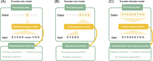
MLM versus autoregressive modeling
An alternative to MLM is autoregressive (left-to-right) modeling, where the model predicts each amino acid conditioned only on the preceding ones:
\[p(x) = \prod_{i=1}^{L} p(x_i \mid x_1, \ldots, x_{i-1})\]Models such as ProGen and ProtGPT2 use this approach. Autoregressive modeling is natural for generation tasks—you sample one amino acid at a time and build a sequence from left to right. However, for understanding tasks (embedding extraction, property prediction, mutation scoring), MLM is generally preferred because it produces bidirectional representations. Each position is influenced by context on both sides, not just the left.
2. ESM-2 Architecture and Model Family
ESM-2 (Evolutionary Scale Modeling 2), developed by researchers at Meta AI, is the current state of the art among protein language models [b]. It combines the Transformer architecture with large-scale training on protein sequence databases, producing representations that capture evolutionary, structural, and functional information.
Training data
ESM-2 was trained on UniRef50, a clustered version of the UniProt database containing roughly 60 million representative protein sequences. Clustering at 50% sequence identity ensures that the training set is diverse: no two sequences in UniRef50 share more than half their residues2.
The Transformer backbone
ESM-2 is built on the Transformer architecture introduced in Lecture 1. The core component is the self-attention mechanism, which allows each position in the sequence to attend to every other position:
\[\text{Attention}(Q, K, V) = \text{softmax}\!\left(\frac{QK^{T}}{\sqrt{d_k}}\right) V\]Here \(Q\), \(K\), and \(V\) are the query, key, and value matrices, obtained by projecting the input embeddings through learned weight matrices \(W_Q\), \(W_K\), and \(W_V\). The scalar \(d_k\) is the dimension of the key vectors; dividing by \(\sqrt{d_k}\) prevents the dot products from growing too large before the softmax.
This mechanism is essential for proteins. Amino acids that are far apart in sequence—say, positions 10 and 150—may be in direct physical contact in the folded structure. A model limited to local context would miss such long-range interactions entirely. Attention connects every position to every other position in a single layer.
ESM-2 uses multi-head attention, splitting the representation into multiple independent attention “heads” that each learn different types of relationships (sequential proximity, co-evolutionary coupling, structural contacts, etc.).
Architectural refinements
ESM-2 incorporates three refinements over a vanilla Transformer:
Rotary Position Embeddings (RoPE). Instead of adding fixed or learned position embeddings to the input, RoPE encodes relative positions by rotating the query and key vectors. This helps the model generalize to sequences longer than those seen during training, because the attention score between two positions depends on their relative distance rather than their absolute positions.
Pre-layer normalization. Layer normalization is applied before the attention and feedforward operations, rather than after. This simple change stabilizes training, especially for very deep models with dozens of layers.
SwiGLU activation. The feedforward sublayers use SwiGLU instead of the standard ReLU or GELU. SwiGLU combines the Swish activation3 with a linear gating mechanism, providing more expressive nonlinear transformations:
import torch.nn as nn

class SwiGLU(nn.Module):
    """
    SwiGLU activation for Transformer feedforward layers.

    Given hidden state x of dimension hidden_size, SwiGLU computes:
        output = W3 * (SiLU(W1 * x) * W2 * x)
    where W1, W2 project to intermediate_size and W3 projects back.
    """
    def __init__(self, hidden_size, intermediate_size):
        super().__init__()
        self.w1 = nn.Linear(hidden_size, intermediate_size, bias=False)
        self.w2 = nn.Linear(hidden_size, intermediate_size, bias=False)
        self.w3 = nn.Linear(intermediate_size, hidden_size, bias=False)

    def forward(self, x):
        return self.w3(nn.functional.silu(self.w1(x)) * self.w2(x))
The ESM-2 model family
ESM-2 is available in six sizes, offering a tradeoff between performance and computational cost:
| Model | Parameters | Layers | Embedding dim | Typical use case |
|---|---|---|---|---|
| ESM-2 8M | 8M | 6 | 320 | Quick prototyping, CPU-friendly |
| ESM-2 35M | 35M | 12 | 480 | Lightweight experiments |
| ESM-2 150M | 150M | 30 | 640 | Good accuracy-cost balance |
| ESM-2 650M | 650M | 33 | 1280 | High performance, fits on a single GPU |
| ESM-2 3B | 3B | 36 | 2560 | Near-state-of-the-art results |
| ESM-2 15B | 15B | 48 | 5120 | Maximum performance, requires multi-GPU |
For most research applications, the 650M-parameter model (denoted esm2_t33_650M_UR50D) provides the best balance. It runs comfortably on a single NVIDIA A100 or even a consumer RTX 3090, and its 1280-dimensional embeddings are nearly as informative as those from the 3B or 15B models.
What does ESM-2 learn?
Without any supervision beyond the MLM objective, ESM-2 representations encode:
- Secondary structure.4 Residues in alpha-helices, beta-sheets, and loops occupy distinct regions of embedding space.
- Solvent accessibility. Buried (hydrophobic core) and exposed (surface) residues are readily distinguishable.
- Functional sites. Active-site residues, metal-binding sites, and other functional motifs have characteristic embedding signatures.
- Evolutionary conservation. Highly conserved positions produce embeddings distinct from variable ones.
- Structural contacts. Positions that are close in three-dimensional space have correlated embeddings, even when far apart in sequence.
These properties emerge from learning to predict masked amino acids. The model is never told about structure, function, or conservation; it discovers them because they are encoded in the statistical patterns of protein sequences.
3. Extracting ESM-2 Embeddings
For a protein of length \(L\) processed by the 650M model, the output is a matrix of shape \((L, 1280)\): one 1280-dimensional vector for each amino acid position. A single summary vector for the whole sequence is obtained by mean pooling across residue positions.
import torch
import esm

def extract_esm_embeddings(sequences, model_name="esm2_t33_650M_UR50D"):
    """
    Extract ESM-2 embeddings for a list of protein sequences.

    Args:
        sequences: List of (label, sequence_string) tuples.
            Example: [("lysozyme", "MKALIVLGL..."), ("GFP", "MSKGEEL...")]
        model_name: Which ESM-2 checkpoint to use.

    Returns:
        Dictionary mapping each label to:
            - 'per_residue': Tensor of shape [L, 1280], one vector per position
            - 'mean': Tensor of shape [1280], the mean-pooled representation
    """
    # Load model and alphabet (tokenizer)
    model, alphabet = esm.pretrained.load_model_and_alphabet(model_name)
    batch_converter = alphabet.get_batch_converter()
    model.eval()

    device = torch.device("cuda" if torch.cuda.is_available() else "cpu")
    model = model.to(device)

    # Tokenize: converts amino acid strings to integer token IDs
    batch_labels, batch_strs, batch_tokens = batch_converter(sequences)
    batch_tokens = batch_tokens.to(device)

    # Forward pass: request representations from the last layer (layer 33)
    with torch.no_grad():
        results = model(
            batch_tokens,
            repr_layers=[33],      # extract from layer 33
            return_contacts=True   # also compute attention-based contacts
        )

    token_embeddings = results["representations"][33]

    # Package results, trimming the special BOS/EOS tokens
    embeddings = {}
    for i, (label, seq) in enumerate(sequences):
        seq_len = len(seq)
        # Positions 1 through seq_len correspond to actual residues
        # (position 0 is the BOS token)
        per_res = token_embeddings[i, 1:seq_len + 1].cpu()   # [L, 1280]
        embeddings[label] = {
            'per_residue': per_res,
            'mean': per_res.mean(dim=0),                       # [1280]
        }

    return embeddings

# --- Example usage ---
# seqs = [("T4_lysozyme", "MNIFEMLRIDE...")]
# emb = extract_esm_embeddings(seqs)
# print(emb["T4_lysozyme"]["mean"].shape)   # torch.Size([1280])
These embeddings can then serve as input features for any downstream predictor—a linear classifier, a small feedforward network, or a more complex model. In many benchmarks, simply training a logistic regression on ESM-2 mean-pooled embeddings outperforms hand-crafted feature pipelines that took decades to develop.
4. Zero-Shot Mutation Scoring
The procedure for zero-shot mutation prediction was described conceptually in Lecture 5. The implementation is straightforward: mask the position of interest, run the forward pass, and compare log-probabilities.
import torch

def predict_mutation_effect(sequence, position, original_aa, mutant_aa,
                            model, alphabet):
    """
    Score a single amino acid substitution using ESM-2 log-likelihood ratio.

    Args:
        sequence: Wild-type amino acid string (e.g., "MKTLLILAVVA").
        position: 0-indexed position of the mutation.
        original_aa: Single-letter code of the wild-type amino acid.
        mutant_aa: Single-letter code of the mutant amino acid.
        model: Loaded ESM-2 model (in eval mode).
        alphabet: ESM-2 alphabet object.

    Returns:
        float: Log-likelihood ratio.
            Positive  -> mutation may be tolerated or favorable.
            Negative  -> mutation is likely deleterious.
    """
    batch_converter = alphabet.get_batch_converter()

    # Create the masked sequence by replacing position i with <mask>
    seq_list = list(sequence)
    seq_list[position] = '<mask>'
    masked_seq = ''.join(seq_list)

    # Tokenize and run the model
    _, _, tokens = batch_converter([("seq", masked_seq)])
    tokens = tokens.to(next(model.parameters()).device)

    with torch.no_grad():
        logits = model(tokens)["logits"]

    # Convert logits to log-probabilities at the masked position
    # Note: position + 1 because the first token is the BOS token
    log_probs = torch.log_softmax(logits[0, position + 1], dim=-1)

    # Look up indices for the wild-type and mutant amino acids
    wt_idx = alphabet.get_idx(original_aa)
    mt_idx = alphabet.get_idx(mutant_aa)

    # Return the log-likelihood ratio
    return (log_probs[mt_idx] - log_probs[wt_idx]).item()
A positive score means the model considers the mutant amino acid more likely than the wild type at that position. A negative score suggests the mutation is deleterious. Studies have shown that these scores correlate well with experimentally measured fitness values from deep mutational scanning experiments [e].
5. Fine-Tuning Classifiers
Fine-tuning adapts pretrained ESM-2 representations to a specific task by adding a lightweight classification head and optionally updating the backbone.
Sequence classification
For tasks that assign a single label to an entire protein—subcellular localization, enzyme class, thermostability—a classification head operates on the mean-pooled embedding:
import torch.nn as nn

class ESMClassifier(nn.Module):
    """
    Sequence-level classifier built on top of ESM-2 embeddings.

    Architecture:
        ESM-2 backbone -> mean pooling -> dropout -> MLP -> class logits
    """
    def __init__(self, esm_model, hidden_dim=1280, num_classes=10,
                 dropout=0.1):
        super().__init__()
        self.esm = esm_model
        self.dropout = nn.Dropout(dropout)
        self.classifier = nn.Sequential(
            nn.Linear(hidden_dim, hidden_dim // 2),
            nn.ReLU(),
            nn.Dropout(dropout),
            nn.Linear(hidden_dim // 2, num_classes)
        )

    def forward(self, tokens):
        # Extract ESM-2 embeddings from the last Transformer layer
        outputs = self.esm(tokens, repr_layers=[33])
        embeddings = outputs["representations"][33]   # [B, L, 1280]

        # Mean pooling over residue positions (exclude special tokens)
        # Token IDs 0, 1, 2 are padding, BOS, EOS respectively
        mask = (tokens != 0) & (tokens != 1) & (tokens != 2)
        mask = mask.unsqueeze(-1).float()             # [B, L, 1]
        pooled = (embeddings * mask).sum(1) / mask.sum(1)  # [B, 1280]

        return self.classifier(self.dropout(pooled))  # [B, num_classes]
Per-residue prediction
For tasks that require a prediction at every position—secondary structure (helix / sheet / coil), binding-site detection, disorder prediction—a classifier is applied independently to each residue embedding:
class ESMTokenClassifier(nn.Module):
    """
    Per-residue classifier built on ESM-2 embeddings.

    Useful for secondary structure prediction (3 classes: H, E, C),
    binding site detection, or disorder prediction.
    """
    def __init__(self, esm_model, hidden_dim=1280, num_labels=3):
        super().__init__()
        self.esm = esm_model
        self.classifier = nn.Sequential(
            nn.Linear(hidden_dim, hidden_dim // 4),
            nn.ReLU(),
            nn.Linear(hidden_dim // 4, num_labels)
        )

    def forward(self, tokens):
        outputs = self.esm(tokens, repr_layers=[33])
        embeddings = outputs["representations"][33]   # [B, L, 1280]
        return self.classifier(embeddings)            # [B, L, num_labels]
Full fine-tuning versus frozen backbone
Two strategies bound the spectrum. Freezing all ESM-2 parameters and training only the classification head is fast and memory-efficient, but the representations are not adapted to the task. Full fine-tuning—updating all parameters—typically gives the best accuracy but is expensive and risks catastrophic forgetting.
A practical middle ground: freeze most layers and fine-tune the last few, or use LoRA.
6. LoRA: Efficient Adaptation
Full fine-tuning of a 650M-parameter model requires storing optimizer states and gradients for every parameter, which can demand 10–20 GB of GPU memory. For the 3B or 15B variants, full fine-tuning is out of reach for most research labs.
Low-Rank Adaptation (LoRA) offers an elegant solution [c].
The key insight
During fine-tuning, the weight updates \(\Delta W\) are typically low-rank. That is, the changes needed to adapt a pretrained model to a new task can be captured by a matrix of much lower rank than the original weight matrix.
The formulation
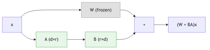
For a pretrained weight matrix \(W \in \mathbb{R}^{d \times k}\), LoRA decomposes the update into two small matrices:
- \(B \in \mathbb{R}^{d \times r}\) (the “down-projection”)
- \(A \in \mathbb{R}^{r \times k}\) (the “up-projection”)
where \(r\) is the rank, a hyperparameter typically set to 4, 8, or 16. The adapted weight matrix is:
\[W_{\text{adapted}} = W_{\text{original}} + BA\]During the forward pass, the output for input \(x\) is:
\[h = W_{\text{original}} \cdot x + \frac{\alpha}{r} \cdot B A \cdot x\]The scalar \(\alpha\) (often called lora_alpha) controls the magnitude of the adaptation relative to the original weights. The ratio \(\alpha / r\) serves as a learning rate scaling factor for the LoRA branch.
Why LoRA works
Massive parameter reduction. For a 1280-by-1280 weight matrix (1,638,400 parameters), LoRA with \(r = 8\) introduces only \(1280 \times 8 + 8 \times 1280 = 20{,}480\) trainable parameters—a 80-fold reduction. Across an entire model, the total trainable parameter count drops to less than 1% of the original.
Memory efficiency. Only the small LoRA matrices require optimizer states and gradients. The original model weights remain frozen in memory but do not need gradient storage.
No catastrophic forgetting. Because the original weights are untouched, the model retains its general-purpose capabilities. Removing the LoRA adapter restores the original model exactly.
Easy task switching. Different LoRA adapters (one per task) can be swapped in and out without reloading the base model. This enables efficient multi-task deployment.
Implementation from scratch
import math
import torch
import torch.nn as nn

class LoRALayer(nn.Module):
    """
    Low-Rank Adaptation wrapper around a frozen linear layer.

    Args:
        original_layer: The pretrained nn.Linear to adapt.
        r: Rank of the low-rank matrices (default 8).
        alpha: Scaling factor (default 16).
        dropout: Dropout rate on the LoRA branch (default 0.1).
    """
    def __init__(self, original_layer, r=8, alpha=16, dropout=0.1):
        super().__init__()
        self.original_layer = original_layer
        self.r = r
        self.alpha = alpha

        in_features = original_layer.in_features
        out_features = original_layer.out_features

        # Freeze the original weights
        for param in self.original_layer.parameters():
            param.requires_grad = False

        # LoRA matrices: A is initialized with Kaiming, B with zeros
        # This ensures the LoRA branch outputs zero at the start of training
        self.lora_A = nn.Parameter(torch.zeros(r, in_features))
        self.lora_B = nn.Parameter(torch.zeros(out_features, r))
        nn.init.kaiming_uniform_(self.lora_A, a=math.sqrt(5))
        nn.init.zeros_(self.lora_B)

        self.dropout = nn.Dropout(dropout)
        self.scaling = alpha / r

    def forward(self, x):
        # Original (frozen) forward pass
        result = self.original_layer(x)

        # LoRA branch: x -> dropout -> A^T -> B^T -> scale
        lora_out = self.dropout(x) @ self.lora_A.T @ self.lora_B.T
        return result + lora_out * self.scaling
Using LoRA with the PEFT library
In practice, the peft library from Hugging Face makes applying LoRA straightforward. LoRA is typically applied to the query and value projection matrices in each attention layer, which have been empirically found to benefit most from adaptation:
from transformers import EsmForSequenceClassification
from peft import get_peft_model, LoraConfig, TaskType

def create_lora_model(model_name, num_labels, r=8, alpha=16):
    """
    Wrap an ESM-2 model with LoRA adapters using Hugging Face PEFT.

    Args:
        model_name: HuggingFace model ID, e.g. "facebook/esm2_t33_650M_UR50D"
        num_labels: Number of output classes.
        r: LoRA rank.
        alpha: LoRA scaling factor.

    Returns:
        PEFT-wrapped model with only LoRA parameters trainable.
    """
    # Load the base ESM-2 model with a classification head
    model = EsmForSequenceClassification.from_pretrained(
        model_name, num_labels=num_labels
    )

    # Configure LoRA: target the attention projection matrices
    lora_config = LoraConfig(
        task_type=TaskType.SEQ_CLS,
        r=r,
        lora_alpha=alpha,
        lora_dropout=0.1,
        target_modules=["query", "key", "value"],
        bias="none"
    )

    peft_model = get_peft_model(model, lora_config)

    # Print summary: expect ~0.1-0.5% trainable parameters
    peft_model.print_trainable_parameters()
    return peft_model

# Example:
# model = create_lora_model("facebook/esm2_t33_650M_UR50D", num_labels=2)
# Output: "trainable params: 1,327,106 || all params: 652,528,898 || trainable%: 0.20"
LoRA has democratized fine-tuning of large protein language models. Tasks that once required clusters of A100 GPUs can now be performed on a single consumer-grade GPU with 12–16 GB of memory.
7. ESMFold: Architecture and Code
Architecture
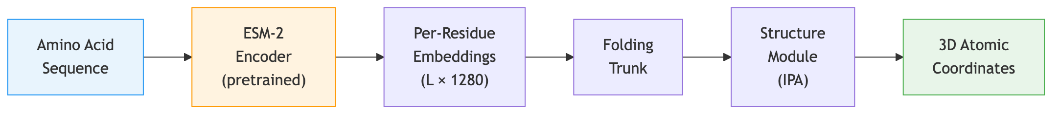
ESMFold takes a protein sequence, passes it through the ESM-2 backbone to produce per-residue embeddings, and then feeds those embeddings into a structure prediction module that generates atomic coordinates. The structure module is similar to the one used in AlphaFold2, operating on pairwise representations and iteratively refining coordinates.
The key difference from AlphaFold2: ESMFold requires only a single sequence, not a multiple sequence alignment (MSA). The ESM-2 embeddings already encode the evolutionary information that AlphaFold2 extracts from the MSA, because the language model has internalized this information during pretraining. This makes ESMFold dramatically faster—seconds per structure instead of minutes.
Code: predicting structure with ESMFold
import torch
import esm

def predict_structure(sequence):
    """
    Predict protein 3D structure from a single amino acid sequence.

    Args:
        sequence: Amino acid string (e.g., "MKTLLILAVVA...").

    Returns:
        PDB-formatted string containing the predicted atomic coordinates.
    """
    # Load the ESMFold model
    model = esm.pretrained.esmfold_v1()
    model = model.eval()

    if torch.cuda.is_available():
        model = model.cuda()

    # Predict structure (returns a PDB string)
    with torch.no_grad():
        pdb_string = model.infer_pdb(sequence)

    return pdb_string

# Save to file and visualize in PyMOL, ChimeraX, or Mol*:
# with open("predicted.pdb", "w") as f:
#     f.write(predict_structure("MKTLLILAVVA..."))
Performance
On the CAMEO benchmark (blind structure prediction), ESMFold achieves accuracy competitive with AlphaFold2 for many protein domains, especially those with abundant homologs in the training set. For proteins with few known relatives—so-called “orphan” or “dark” proteins—ESMFold’s accuracy can drop, because the language model has less evolutionary context to draw on.
The success of ESMFold demonstrates something profound: the statistical patterns in sequence data encode sufficient information to recover three-dimensional structure. The grammar of proteins is inseparable from their physics.
8. Attention Maps as Structure Windows
The attention mechanism in ESM-2 is not just a computational tool; it provides an interpretable window into what the model has learned.
Attention correlates with structural contacts
Each attention head computes a matrix of attention weights, one weight for every pair of positions in the sequence. Research has shown that these attention patterns correlate with residue-residue contacts in the three-dimensional structure [a]. Positions that are close in space (within about 8 Angstroms) tend to attend strongly to each other, even when they are far apart in sequence.
This means the model has discovered, purely from sequence statistics, the same principle that underlies evolutionary coupling analysis: co-evolving residues are in structural contact.
Code: extracting and processing attention maps
import torch

def extract_attention_maps(model, tokens, layer=-1):
    """
    Extract attention maps from a specific ESM-2 layer.

    Args:
        model: Loaded ESM-2 model.
        tokens: Tokenized input (shape [1, L]).
        layer: Which layer to extract from (-1 = last layer).

    Returns:
        Attention tensor of shape [num_heads, L, L].
    """
    with torch.no_grad():
        outputs = model(tokens, return_contacts=True)

    attentions = outputs["attentions"]
    return attentions[layer][0]   # [num_heads, L, L]


def attention_to_contacts(attention, threshold=0.5):
    """
    Derive a predicted contact map from attention weights.

    Steps:
        1. Average over attention heads.
        2. Symmetrize (contacts are undirected).
        3. Apply APC (Average Product Correction) to remove background.
        4. Threshold to get binary predictions.

    Args:
        attention: Tensor of shape [num_heads, L, L].
        threshold: Cutoff for binary contact prediction.

    Returns:
        Binary contact map of shape [L, L].
    """
    # Average over heads
    attn_mean = attention.mean(0)                     # [L, L]

    # Symmetrize: contacts are undirected
    attn_sym = (attn_mean + attn_mean.T) / 2

    # APC correction: remove phylogenetic background signal
    row_mean = attn_sym.mean(1, keepdim=True)
    col_mean = attn_sym.mean(0, keepdim=True)
    overall_mean = attn_sym.mean()
    apc = (row_mean * col_mean) / overall_mean
    corrected = attn_sym - apc

    return (corrected > threshold).float()
The APC (Average Product Correction) step is borrowed from the evolutionary coupling literature. It removes the background correlation that arises because all positions share a common phylogenetic history, isolating the direct coupling signal that reflects physical contacts.
Different heads, different relationships
Not all attention heads learn the same thing. Studies have found that different heads specialize:
- Some heads capture sequential proximity—attending primarily to nearby residues.
- Some capture long-range contacts—attending to residues that are far in sequence but close in structure.
- Some appear to encode secondary structure periodicity—attending at intervals of 3–4 residues (the pitch of an alpha-helix).
This specialization emerges entirely from the MLM training objective. No structural supervision is provided.
Key Takeaways
-
Masked language modeling learns rich representations from raw sequences without any labels. By predicting masked amino acids, the model implicitly discovers conservation, co-evolution, secondary structure, and functional motifs.
-
ESM-2’s transformer architecture incorporates rotary position embeddings (for length generalization), pre-layer normalization (for training stability), and SwiGLU activations (for expressive feedforward layers). The 650M model provides the best performance-cost tradeoff.
-
Embedding extraction is straightforward: a forward pass through ESM-2 yields per-residue vectors (shape \(L \times 1280\)) and a mean-pooled sequence vector. These serve as drop-in features for any downstream predictor.
-
Zero-shot mutation scoring computes a log-likelihood ratio at a masked position. Positive scores suggest tolerated mutations; negative scores suggest deleterious ones. No task-specific training is needed.
-
Fine-tuning adds a classification head (sequence-level or per-residue) on top of ESM-2 embeddings. Freezing the backbone is fast but suboptimal; full fine-tuning is expensive and risks catastrophic forgetting.
-
LoRA decomposes weight updates into low-rank matrices (\(BA\)), reducing trainable parameters to less than 1% of the original model. This makes fine-tuning feasible on consumer GPUs and eliminates catastrophic forgetting.
-
ESMFold feeds ESM-2 embeddings into a structure module to predict 3D coordinates from a single sequence, bypassing the expensive MSA computation that AlphaFold2 requires.
-
Attention maps correlate with structural contacts. Different heads specialize in sequential proximity, long-range contacts, and secondary structure periodicity—all discovered from the MLM objective alone.
Tasks and applications: Lecture 5 (PLM Tasks) covers what pLMs achieve—the protein-language analogy, zero-shot scoring use cases, clinical variant interpretation, and the ESM Metagenomic Atlas.
Further Reading
- Tasks companion: Lecture 5: PLM Tasks and Applications — what pLMs learn and how they are used in practice
- Code walkthrough: nano-esm2 — build ESM2 from scratch in 288 lines of PyTorch
- Stephen Malina, “Protein Language Models (Part 1)” and “Part 2” — comprehensive review of PLM architectures (ESM-1b, ESM-2, UniRep, CARP) and their scaling behavior.
- Evolutionary Scale, “ESM Cambrian” — official blog on unsupervised protein representation learning at evolutionary scale.
- Evolutionary Scale, “ESM3: Simulating 500 Million Years of Evolution” — multimodal protein language modeling across sequence, structure, and function.
References
[a] Rives, A., Meier, J., Sercu, T., Goyal, S., Lin, Z., Liu, J., Guo, D., Ott, M., Zitnick, C.L., Ma, J., & Fergus, R. (2021). Biological structure and function emerge from scaling unsupervised learning to 250 million protein sequences. Proceedings of the National Academy of Sciences, 118(15), e2016239118.
[b] Lin, Z., Akin, H., Rao, R., Hie, B., Zhu, Z., Lu, W., Smetanin, N., Verkuil, R., Kabeli, O., Shmueli, Y., dos Santos Costa, A., Fazel-Zarandi, M., Sercu, T., Candido, S., & Rives, A. (2023). Evolutionary-scale prediction of atomic-level protein structure with a language model. Science, 379(6637), 1123–1130.
[c] Hu, E.J., Shen, Y., Wallis, P., Allen-Zhu, Z., Li, Y., Wang, S., Wang, L., & Chen, W. (2022). LoRA: Low-Rank Adaptation of Large Language Models. Proceedings of the International Conference on Learning Representations (ICLR).
[d] Elnaggar, A., Heinzinger, M., Dallago, C., Rehawi, G., Wang, Y., Jones, L., Gibbs, T., Feher, T., Angerer, C., Steinegger, M., Bhowmik, D., & Rost, B. (2022). ProtTrans: Toward understanding the language of life through self-supervised learning. IEEE Transactions on Pattern Analysis and Machine Intelligence, 44(10), 7112–7127.
[e] Meier, J., Rao, R., Verkuil, R., Liu, J., Sercu, T., & Rives, A. (2021). Language models enable zero-shot prediction of the effects of mutations on protein function. Advances in Neural Information Processing Systems (NeurIPS), 34, 29287–29303.
-
MLM was introduced by Devlin et al. (2019) as the training objective for BERT. Its application to proteins was pioneered by Rives et al. (2021) in the ESM family. ↩
-
UniRef clusters are created by the UniProt consortium. UniRef50 clusters sequences at 50% identity; UniRef90 at 90%. ESM-2 uses UniRef50 for maximum diversity. ↩
-
Swish, also known as SiLU (Sigmoid Linear Unit), is defined as \(\text{Swish}(x) = x \cdot \sigma(x)\), where \(\sigma\) is the sigmoid function. ↩
-
Secondary structure refers to the local folding patterns within a protein: alpha helices (rod-like coils stabilized by backbone hydrogen bonds), beta sheets (flat structures formed by side-by-side strands), and loops/coils (irregular connecting regions). These are the building blocks that pack together to form the overall 3D shape. ↩