Protein Language Models: Tasks and Applications
This is Lecture 5 (first of two parts) of the Protein & Artificial Intelligence course (Spring 2026), co-taught by Prof. Sungsoo Ahn and Prof. Homin Kim at KAIST. It covers what protein language models achieve and why they work. The companion Lecture 6 covers the how: architecture, training objective, and implementation code.
Introduction
What if amino acid sequences are sentences, and evolution is the author?
This is not a loose metaphor. Over four billion years, natural selection has tested protein sequences against the harshest possible critic: survival. The sequences we observe today are the ones that fold correctly, carry out their functions, and keep their organisms alive. They are, in a precise statistical sense, the grammatically correct sentences in the language of life.
Protein language models (pLMs) take this analogy seriously. They train on hundreds of millions of protein sequences, learning representations that encode evolutionary constraints, structural contacts, and functional motifs—all without a single experimental label.
The payoff is broad. ESM-2 embeddings improve virtually every protein-understanding task that has been tested. Zero-shot mutation scoring rivals purpose-built predictors. ESMFold predicts three-dimensional structure from a single sequence, without multiple sequence alignments. Fine-tuning with parameter-efficient adapters makes all of this accessible on a single GPU.
This lecture develops the what and why of protein language models: the conceptual foundations, the tasks they solve, and the practical applications transforming protein science today. Lecture 6 covers the how: masked language modeling, the ESM-2 transformer architecture, and the code for embeddings, mutation scoring, fine-tuning, and contact prediction.
Roadmap
| Section | Why it is needed |
|---|---|
| The Protein-Language Analogy | Motivates why NLP techniques transfer to proteins |
| Learning from Evolutionary Experiments | Explains the self-supervised signal hiding in sequence databases |
| The Foundation Model Paradigm | Places pLMs in the broader landscape of pretrain-finetune AI |
| Extracting and Using Embeddings | Shows what per-residue and sequence-level representations capture |
| Zero-Shot Mutation Prediction | Demonstrates label-free fitness estimation |
| Fine-Tuning for Specific Tasks | Adapts pLM representations to labeled datasets |
| How People Use PLMs in Practice | Surveys real-world deployments from metagenomics to the clinic |
| ESMFold: From Embeddings to Structure | Shows that embeddings encode enough to predict 3D shape |
| The Broader pLM Landscape | Surveys alternative models and their niches |
| Practical Considerations | Guides model selection, memory budgets, and batch processing |
1. The Protein-Language Analogy
Before introducing any formulas, consider proteins and natural language side by side.
In English, words combine into sentences according to grammatical rules. Some word combinations are meaningful; most are not. The meaning of a word depends on context: “bank” means one thing in “river bank” and another in “bank account.” Synonyms exist—words that differ in form but serve similar functions. And language evolves over time while preserving core structural principles.
Proteins share every one of these properties.
Amino acids are words. Twenty distinct chemical building blocks serve as the vocabulary1. Each has a characteristic side chain that determines its chemical personality: hydrophobic, charged, polar, aromatic, and so on.
Protein sequences are sentences. A linear chain of amino acids encodes a specific three-dimensional structure and biological function, just as a sentence encodes meaning through a linear arrangement of words.
Biochemical constraints are grammar. Most random strings of amino acids will not fold into stable structures. They aggregate, misfold, or fail to function. The sequences we observe in nature have passed through the filter of natural selection, which permits only “grammatically correct” protein sentences to survive. This is analogous to the observation that most random strings of English letters do not form valid sentences.
Context determines meaning. The same amino acid plays different roles depending on its neighbors. A hydrophobic2 residue buried in the protein core contributes to thermodynamic stability. The same residue on the protein surface might create a binding interface3 for a partner protein. Histidine can act as a catalytic acid-base in an enzyme active site4, coordinate a metal ion, or play a purely structural role—all depending on its sequence context.
Conservative substitutions are synonyms. Leucine and isoleucine are both large, branched, hydrophobic amino acids. In many sequence positions, one can replace the other without destroying function, just as “big” and “large” can often substitute for each other in English. This is not random; it reflects the underlying biochemistry, the semantics of the protein language.
Co-evolution mirrors co-occurrence. In English, “salt” frequently co-occurs with “pepper.” In proteins, pairs of residues that are in physical contact in the three-dimensional structure tend to mutate in a correlated fashion5. If one partner changes, the other compensates to maintain the interaction. This co-evolutionary signal is the protein equivalent of word co-occurrence statistics.
The following table summarizes the correspondence:
| Natural Language | Protein Language |
|---|---|
| Words / tokens | Amino acids |
| Sentences | Protein sequences |
| Grammar rules | Biochemical and physical constraints |
| Semantics (meaning) | Three-dimensional structure and function |
| Synonyms | Functionally equivalent substitutions (e.g., Leu / Ile) |
| Word co-occurrence | Co-evolution of contacting residues |
| Corpus of text | Protein sequence databases (UniProt, UniRef) |
This structural parallel suggests a concrete research strategy: apply the same machine learning techniques that have transformed natural language processing to protein sequences. As we will see, the results exceed what the analogy alone might lead us to expect.
2. Learning from Billions of Evolutionary Experiments
Why should a model trained to fill in missing amino acids learn anything useful about protein biology?
The answer lies in what the training data actually represents. The UniProt database contains over 200 million protein sequences, and metagenomic surveys are adding billions more. Each of these sequences is the outcome of a successful evolutionary experiment—a design that folds, functions, and keeps its organism alive. The sequences that failed these tests are absent from our databases because their organisms did not survive.
When a model sees thousands of sequences from a single protein family, it observes statistical regularities that reflect genuine biological constraints:
- Absolute conservation. Some positions never change across the entire family. These are almost always critical for structure or function—active-site residues, disulfide-bonding cysteines6, glycine residues in tight turns.
- Constrained variation. Some positions vary, but only within a restricted class of amino acids. A position that accepts leucine, isoleucine, and valine—but never aspartate—is almost certainly in the hydrophobic core of the protein.
- Correlated variation. Some positions change together. When residue 42 mutates from a small side chain to a large one, residue 108 compensates by mutating from large to small. This co-evolutionary signal reveals that the two positions are in spatial contact7.
The model does not need to be told about any of these concepts. It discovers them by learning to predict masked amino acids accurately. This is the core insight of self-supervised learning applied to biology: the sequences themselves contain the supervision.
The scale of available data makes this approach particularly powerful. Hundreds of millions of protein sequences represent far more training data than exists for most natural language tasks. Each sequence is the product of a distinct evolutionary lineage, providing diverse perspectives on what works in protein design. By learning from this vast corpus, protein language models capture knowledge that would be impossible to encode by hand.
3. The Foundation Model Paradigm
Protein language models are an instance of a broader idea that has reshaped machine learning: the foundation model.
What is a foundation model?
A foundation model is a large neural network trained on a broad, unlabeled dataset using a self-supervised objective, then adapted to specific tasks through fine-tuning or prompting. The term was coined by the Stanford HAI group in 2021, but the pattern emerged earlier with BERT (2018) and GPT-2 (2019). The defining characteristic is task generality: a single pretrained model serves as the starting point for many downstream applications, rather than training a specialist model from scratch for each one.
In natural language processing, the progression was clear. Before BERT, each NLP task—sentiment analysis, named entity recognition, question answering—required its own architecture and its own labeled dataset. BERT changed the economics: pretrain once on a massive text corpus, fine-tune cheaply on each task. GPT extended this further, showing that sufficiently large models could perform new tasks with no fine-tuning at all (zero-shot and few-shot inference).
The pretrain-finetune paradigm
The two-stage workflow follows a consistent template:
Stage 1: Pretraining. Train a large model on a massive unlabeled corpus with a self-supervised objective. For text, this means predicting masked words (BERT) or the next word (GPT). For proteins, this means predicting masked amino acids (ESM-2) or the next amino acid (ProGen). The model learns general-purpose representations—statistical regularities that encode syntax, semantics, and world knowledge in the text case, or evolutionary constraints, structural contacts, and functional motifs in the protein case.
Stage 2: Adaptation. Take the pretrained model and adapt it to a specific task. This can be full fine-tuning (update all parameters on labeled data), parameter-efficient fine-tuning (update a small fraction of parameters, e.g., with LoRA), linear probing (train only a classifier head on frozen embeddings), or zero-shot inference (use the pretrained model’s predictions directly, with no task-specific training at all).
The power of this paradigm lies in data efficiency. Pretraining absorbs the information contained in hundreds of millions of unlabeled sequences. Fine-tuning then needs only hundreds or thousands of labeled examples to steer the model toward a specific task, because the hard work of learning general representations is already done.
Why protein sequences are ideal for self-supervised learning
Several properties make protein sequences a near-perfect fit for the foundation model paradigm:
Abundance without labels. UniRef contains over 200 million non-redundant protein sequences. The ESM Metagenomic Atlas adds 2.3 billion more from environmental samples. By contrast, even the largest labeled protein datasets—deep mutational scans, structure databases, functional annotations—contain at most tens of thousands of entries. Self-supervised learning bridges this gap by extracting supervision from the sequences themselves.
Each sequence is an evolutionary experiment. Unlike internet text, where a sentence might be grammatically correct but factually wrong, every natural protein sequence has been validated by the most stringent quality assurance process on Earth: billions of years of natural selection. A sequence in UniProt works—it folds, functions, and contributed to its organism’s survival. This means the training data is information-dense; every sequence encodes real biophysical constraints.
Fixed vocabulary, variable length. The 20-amino-acid alphabet is smaller and more chemically interpretable than the ~50,000-token vocabularies typical of NLP models. Sequence lengths range from tens to thousands of residues, but the vocabulary is constant. This simplifies tokenization (each amino acid is one token) and makes the masked prediction task crisp: predict one of 20 classes at each position.
Hierarchical structure. Like natural language, proteins have structure at multiple scales: local motifs (helices, sheets), domains, multi-domain architectures, and complexes. A model that learns to predict masked residues must implicitly capture all these levels, because they all constrain which amino acids can appear at a given position.
Positioning pLMs in the landscape of protein AI
Protein AI methods span a spectrum from physics-based to data-driven:
| Approach | Input | What it captures | Example |
|---|---|---|---|
| Molecular dynamics | Atomic coordinates + force field | Physical forces | GROMACS, OpenMM |
| Homology modeling | MSA + template structures | Evolutionary conservation | SWISS-MODEL |
| Co-evolution methods | MSA | Pairwise correlations | EVcouplings, GREMLIN |
| Protein language models | Raw sequences | All of the above, implicitly | ESM-2, ProtTrans |
| Structure prediction | Sequence (+ MSA) | 3D coordinates | AlphaFold2, ESMFold |
Protein language models sit at a unique point: they take the simplest possible input (a raw amino acid sequence), require no alignments or templates, and produce representations rich enough to support tasks ranging from function prediction to structure determination. They are not the final answer—physics-based methods remain essential for dynamics, and AlphaFold2 still outperforms ESMFold on hard targets—but they provide the most versatile starting point available.
4. Extracting and Using Embeddings
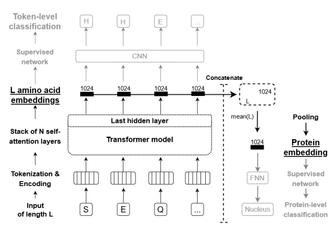
One of the most practical applications of a pretrained pLM is embedding extraction: passing a protein sequence through the model and collecting the internal representations for downstream tasks.
Per-residue embeddings
For a protein of length \(L\) processed by the 650M-parameter ESM-2 model, the output is a matrix of shape \((L, 1280)\): one 1280-dimensional vector for each amino acid position. Each vector encodes information about that residue in the context of the full sequence—its local chemical environment, its evolutionary conservation, and its likely structural role.
These per-residue vectors are the input for tasks that require a prediction at every position: secondary structure classification (helix / sheet / coil), binding-site identification, disorder prediction, post-translational modification site detection.
Sequence-level embeddings
Tasks that assign a single label to an entire protein—subcellular localization, enzyme class, thermostability, solubility—require a single vector representing the whole sequence. The standard approach is mean pooling: averaging across all \(L\) residue vectors to produce one 1280-dimensional summary. Alternatives include using the embedding at a special beginning-of-sequence token, or attention-weighted pooling that gives higher weight to positions the model deems important.
Mean pooling is simple and works well in practice. On many benchmarks, training a logistic regression on mean-pooled ESM-2 embeddings outperforms hand-crafted feature pipelines that took decades to develop.
Downstream tasks
The embedding-then-classify pattern is remarkably general. The same pretrained model, without any modification, feeds into classifiers for:
- Secondary structure prediction (3-class per-residue: H, E, C).
- Subcellular localization (10+ classes per-sequence: nucleus, cytoplasm, membrane, etc.).
- Remote homology detection (fold-level classification from sequence alone).
- Fluorescence and stability prediction from deep mutational scanning data.
- Protein-protein interaction prediction using concatenated or pairwise embeddings.
The quality of these embeddings improves with model size, following scaling laws similar to those observed in NLP. The 650M model captures most of the performance gains; the 3B and 15B models add marginal improvements at substantially higher cost.
5. Zero-Shot Mutation Prediction
Perhaps the most striking capability of protein language models is zero-shot prediction of mutational effects. Without any fine-tuning or task-specific labels, ESM-2 can estimate whether a single amino acid substitution is likely to be beneficial, neutral, or deleterious.
The intuition
The model has learned the distribution of natural, functional protein sequences. A mutation that pushes a sequence away from this distribution—into regions of sequence space that evolution has avoided—is likely to be harmful. A mutation that keeps the sequence within the distribution is likely to be tolerated.
The procedure
Let \(s\) be the wild-type sequence, and suppose we want to score the mutation from amino acid \(a_{\text{wt}}\) to \(a_{\text{mut}}\) at position \(i\).
- Mask position \(i\) in the sequence, replacing it with a mask token.
- Run the masked sequence through the model to obtain predicted probabilities over the 20 amino acids at position \(i\).
- Compare the log-probability of the mutant amino acid to the log-probability of the wild-type amino acid:
A positive score means the model considers the mutant amino acid more likely than the wild type at that position, suggesting the mutation may be tolerated or even beneficial. A negative score means the mutation moves away from the learned evolutionary distribution, suggesting it may be deleterious.
Why does this work?
The model has absorbed the outcomes of hundreds of millions of evolutionary experiments. At any given position, it has seen which amino acids appear across all known homologs8 and which are absent.
Mutations to amino acids that never appear at a position in any natural sequence receive low probability and negative scores. Mutations to amino acids that are common at that position receive high probability and scores near zero or positive.
This captures the essence of evolutionary constraint. Studies have shown that ESM-2 zero-shot scores correlate well with experimentally measured mutational fitness values from deep mutational scanning9 (DMS) experiments [e].
In many cases, the zero-shot predictor matches or exceeds the performance of supervised methods trained directly on experimental data.
Practical significance
Experimental measurement of mutational effects is expensive and slow. A typical DMS experiment covers all single-point mutations of a single protein, requires specialized equipment, and can take months. Zero-shot pLM scoring provides an instant, free estimate that can:
- Prioritize mutations for experimental testing.
- Flag potentially harmful variants in clinical genomics.
- Guide protein engineering campaigns toward productive regions of sequence space.
6. Fine-Tuning for Specific Tasks
While zero-shot capabilities are impressive, fine-tuning ESM-2 on task-specific labeled data can further improve performance. Fine-tuning adapts the pretrained representations to a particular problem, learning which aspects of the embeddings are most relevant for the task at hand.
Sequence classification
For tasks that assign a single label to an entire protein—predicting subcellular localization, enzyme class, or thermostability—the standard approach adds a classification head on top of the mean-pooled embedding. The head is typically a small feedforward network: one or two hidden layers with dropout, producing class logits. The ESM-2 backbone provides a 1280-dimensional pooled vector; the classification head maps this to the number of output classes.
Per-residue prediction
For tasks that require a prediction at every position—secondary structure classification, binding-site detection, disorder prediction—a classifier is applied independently to each residue embedding. The per-residue classifier is structurally similar to the sequence-level one, but operates on each of the \(L\) position vectors rather than on the pooled summary.
Full fine-tuning versus frozen backbone
Two strategies bound the spectrum:
- Frozen backbone. Freeze all ESM-2 parameters and train only the classification head. This is fast and requires minimal GPU memory, but the representations are not adapted to the task.
- Full fine-tuning. Update all parameters, including the ESM-2 backbone. This typically gives the best performance but is computationally expensive and risks catastrophic forgetting: the model may lose its general-purpose capabilities as it overfits to the small task-specific dataset.
A middle ground often works best: freeze most of the ESM-2 layers and fine-tune only the last few, along with the classification head. Or, better yet, use LoRA—a parameter-efficient adaptation method that reduces trainable parameters to less than 1% of the original model while avoiding catastrophic forgetting entirely (covered in Lecture 6).
7. How People Use PLMs in Practice
The conceptual tools above—embedding extraction, zero-shot scoring, fine-tuning—translate into concrete workflows across protein science. This section surveys four domains where pLMs are already changing practice.
The ESM Metagenomic Atlas
In 2022, Meta AI applied ESMFold to 2.3 billion metagenomic protein sequences—sequences recovered from environmental DNA samples (ocean water, soil, gut microbiomes) that have never been cultured in a lab. The result is the ESM Metagenomic Atlas: predicted structures for over 617 million proteins, more than tripling the number of known protein structures overnight.
The scale is staggering. The Protein Data Bank, built over 50 years of experimental crystallography and cryo-EM, contains roughly 220,000 structures. AlphaFold DB added 214 million predicted structures from known organisms. The ESM Atlas extends coverage to the vast “dark” proteome—proteins from uncultured organisms that have no close homologs in existing databases.
Many of these predictions reveal novel folds and domain architectures not seen in any characterized organism. Because ESMFold runs on single sequences (no MSA needed), it could process 2.3 billion sequences in a matter of weeks on a GPU cluster—a task that would take years with AlphaFold2’s MSA-dependent pipeline.
The atlas is publicly available at esmatlas.com and has already been used to discover new antibiotic candidates, characterize viral proteins, and identify enzymes for industrial biotechnology.
Clinical variant interpretation
Every human genome contains roughly 10,000 missense variants—amino acid changes relative to the reference sequence. Most are benign; a small fraction cause disease. Distinguishing the two is one of the central challenges of clinical genetics.
Zero-shot pLM scores provide a powerful signal for variant classification. The log-likelihood ratio from ESM-2 (or its predecessor ESM-1b) correlates with pathogenicity: variants at conserved, functionally critical positions receive large negative scores, while variants at tolerant positions score near zero.
Several studies have benchmarked this approach:
- On ClinVar (a curated database of clinically annotated variants), ESM-1b zero-shot scores separate pathogenic from benign variants with an AUC of ~0.85, competitive with supervised methods like PolyPhen-2 and CADD that use dozens of hand-engineered features.
- The 2023 AlphaMissense model from DeepMind combines ESM-style embeddings with AlphaFold structural features to classify 71 million possible human missense variants, achieving 90% precision at 90% recall on held-out ClinVar data.
The advantage of pLM-based scoring is generality: it works for any protein, any variant, with no need for family-specific training data. This makes it especially valuable for rare diseases and understudied proteins where labeled data is scarce.
Protein engineering workflows
Protein engineers use pLMs at multiple stages of the design-build-test cycle:
Embedding-based virtual screening. Given a library of candidate sequences (from directed evolution, computational design, or combinatorial mutagenesis), compute ESM-2 embeddings and train a lightweight predictor on a small set of experimentally characterized variants. This “embed-and-regress” approach typically outperforms sequence-based models (one-hot encoding, k-mer features) because the embeddings already encode structural and evolutionary context. Studies on GFP fluorescence, AAV capsid fitness, and enzyme activity have shown 2–5x improvements in prediction accuracy using pLM embeddings versus raw sequence features.
Zero-shot library design. Before synthesizing any DNA, score all candidate mutations with the pLM log-likelihood ratio. Discard mutations with strongly negative scores (likely deleterious) and prioritize those with neutral or positive scores. This pre-screening can reduce experimental library sizes by 50–80% while retaining most functional variants.
LoRA fine-tuning for specific assays. When a few hundred labeled measurements are available (e.g., from an initial round of directed evolution), fine-tune ESM-2 with LoRA on this data. The adapted model serves as a fitness predictor for the next round of design. Because LoRA trains less than 1% of parameters, this is feasible on a single consumer GPU in under an hour.
Drug discovery and beyond
Pharmaceutical and biotech companies are integrating pLMs into their pipelines:
Target identification. Embed entire proteomes with ESM-2 and cluster by embedding similarity to identify protein families, discover remote homologs of known drug targets, and annotate proteins of unknown function. Embedding-based clustering is faster than sequence alignment (BLAST) and captures functional relationships that sequence identity misses.
Epitope and binding-site prediction. Per-residue embeddings feed into classifiers that predict antibody epitopes (surface regions recognized by antibodies) and small-molecule binding pockets. These predictions guide vaccine design, antibody engineering, and structure-based drug design even when experimental structures are unavailable.
Enzyme discovery for green chemistry. Mining metagenomic databases with pLM embeddings has identified novel plastic-degrading enzymes (PETases), carbon-fixing enzymes, and biofuel-pathway enzymes. The ESM Metagenomic Atlas provides a searchable database of predicted structures for these proteins, accelerating the pipeline from sequence discovery to functional characterization.
Antibody language models. Specialized pLMs trained on antibody sequences (AbLang, AntiBERTa, IgLM) capture the unique evolutionary pressures on immunoglobulin variable regions. These models predict developability (aggregation, viscosity, polyreactivity) and guide humanization of therapeutic antibodies.
The common thread across these applications is that pLM embeddings serve as a universal representation layer: a fixed-dimensional summary of a protein’s identity that plugs into any downstream machine learning pipeline. The days of hand-engineering protein features—amino acid composition, physicochemical descriptors, position-specific scoring matrices—are ending.
8. ESMFold: From Embeddings to Structure
The ultimate test of whether a language model truly “understands” proteins is whether its representations contain enough information to predict three-dimensional structure. ESMFold demonstrates that they do [b].
What ESMFold does
ESMFold takes a protein sequence, passes it through the ESM-2 backbone to produce per-residue embeddings, and then feeds those embeddings into a structure prediction module that generates atomic coordinates. The structure module is similar to the one used in AlphaFold2, operating on pairwise representations and iteratively refining coordinates.
The key difference from AlphaFold2
AlphaFold2 requires a multiple sequence alignment (MSA) as input: a collection of evolutionary relatives of the query protein, aligned position by position. Constructing this MSA is computationally expensive, often taking minutes to hours for a single protein.
ESMFold requires only a single sequence. The ESM-2 embeddings already encode the evolutionary information that AlphaFold2 extracts from the MSA, because the language model has internalized this information during pretraining. This makes ESMFold dramatically faster—seconds per structure instead of minutes.
Performance
On the CAMEO benchmark (blind structure prediction), ESMFold achieves accuracy competitive with AlphaFold2 for many protein domains, especially those with abundant homologs in the training set. For proteins with few known relatives—so-called “orphan” or “dark” proteins—ESMFold’s accuracy can drop, because the language model has less evolutionary context to draw on.
The success of ESMFold demonstrates something profound: the statistical patterns in sequence data encode sufficient information to recover three-dimensional structure. The grammar of proteins is inseparable from their physics.
9. The Broader pLM Landscape
ESM-2 is the most widely used protein language model, but it is not the only one. Several alternatives exist, each with distinct strengths.
ProtTrans [d], developed at the Technical University of Munich, offers models based on multiple Transformer architectures—BERT, ALBERT, XLNet, and T5. The ProtT5-XL variant has been particularly popular for per-residue prediction tasks, offering a good balance of performance and efficiency with its encoder-decoder architecture.
ProGen and ProGen2, developed at Salesforce, use autoregressive modeling (left-to-right generation, like GPT). This makes them especially effective for protein design and sequence generation tasks, where sampling new sequences from the learned distribution is the goal.
ProtGPT2 follows a similar autoregressive strategy and has been shown to generate novel protein sequences that fold into stable structures, as validated by AlphaFold2 predictions.
Ankh, developed at TU Munich, offers efficient training strategies that achieve competitive performance with significantly less compute than ESM-2, making pretraining more accessible to resource-constrained groups.
ProteinBERT, developed at Google, incorporates Gene Ontology (GO) annotations during pretraining. By jointly predicting masked amino acids and GO terms, it explicitly learns functional information alongside sequence patterns.
| Model | Training objective | Key strength |
|---|---|---|
| ESM-2 | Masked LM | General-purpose embeddings, wide size range |
| ProtT5-XL | Span denoising (T5-style) | Per-residue tasks, encoder-decoder flexibility |
| ProGen / ProGen2 | Autoregressive LM | Sequence generation and design |
| Ankh | Masked LM | Compute-efficient pretraining |
| ProteinBERT | Masked LM + GO prediction | Function-aware representations |
For general-purpose embedding extraction, ESM-2 remains the default choice due to its strong benchmark performance and the availability of models at multiple scales. For generation tasks, autoregressive models such as ProGen2 are more natural.
10. Practical Considerations
Deploying protein language models in a research workflow involves several practical choices.
Model size selection
- 8M / 35M: Fast inference, CPU-friendly. Good for pipeline prototyping and debugging.
- 150M: Reasonable performance at low cost. Suitable when GPU resources are limited.
- 650M: The recommended default. Fits on a single GPU with 4+ GB VRAM for inference, ~16 GB for LoRA fine-tuning.
- 3B / 15B: Marginal gains over 650M on most tasks. Use when accuracy is paramount and multi-GPU resources are available.
Sequence length
ESM-2 was trained on sequences up to 1024 amino acids. Longer sequences require one of three strategies:
- Truncation: Use only the first 1022 residues (leaving room for BOS/EOS tokens). Information beyond the cutoff is lost.
- Chunking: Split the sequence into overlapping windows, embed each window, and merge the results. Residues in overlapping regions can be averaged.
- Longer-context models: Some newer models support longer sequences natively.
GPU memory budget
| Model | Inference (approx.) | LoRA fine-tuning (approx.) | Full fine-tuning (approx.) |
|---|---|---|---|
| ESM-2 35M | < 1 GB | ~2 GB | ~4 GB |
| ESM-2 150M | ~1 GB | ~4 GB | ~8 GB |
| ESM-2 650M | ~2.5 GB | ~8 GB | ~24 GB |
| ESM-2 3B | ~12 GB | ~24 GB | ~80 GB+ |
Batch processing
When embedding many sequences, group them by length and pad within each batch. The ESM library’s batch converter handles this automatically, but custom pipelines should be careful to avoid excessive padding, which wastes compute.
Reproducibility
Set random seeds and use deterministic CUDA operations when comparing methods. This is especially important for fine-tuning experiments where small differences in initialization can lead to different results.
Key Takeaways
-
Proteins are a language with amino acids as tokens, sequences as sentences, and evolutionary constraints as grammar. This structural parallel justifies applying NLP techniques to protein sequences.
-
Self-supervised learning on sequences discovers conservation, co-evolution, secondary structure, and functional motifs—all without experimental labels. The sequences themselves contain the supervision.
-
The foundation model paradigm (pretrain once, adapt many times) applies powerfully to proteins: 200M+ unlabeled sequences enable general-purpose representations that transfer to any downstream task.
-
ESM-2 embeddings encode evolutionary, structural, and functional information. They serve as drop-in features for downstream prediction, often outperforming hand-crafted feature pipelines.
-
Zero-shot mutation prediction requires no task-specific training. The log-likelihood ratio at a masked position estimates mutational fitness, often matching supervised methods.
-
Real-world applications span the ESM Metagenomic Atlas (617M predicted structures), clinical variant interpretation (AUC ~0.85 on ClinVar), protein engineering (2–5x accuracy gains from pLM embeddings), and drug discovery.
-
ESMFold predicts three-dimensional protein structure from a single sequence in seconds, demonstrating that language model embeddings capture sufficient information to recover 3D shape.
-
The pLM landscape includes encoder models (ESM-2, ProtTrans) for understanding and autoregressive models (ProGen, ProtGPT2) for generation. ESM-2 remains the default for embedding extraction.
Build it yourself: The nano-esm2 code walkthrough implements the architecture from scratch in 288 lines of PyTorch. Two files, no abstractions—fork it, break it, learn from it.
Further Reading
- Implementation companion: Lecture 6: PLM Architecture and Training — masked language modeling, ESM-2 architecture, LoRA, attention maps
- Code walkthrough: nano-esm2 — build ESM2 from scratch in 288 lines of PyTorch
- Stephen Malina, “Protein Language Models (Part 1)” and “Part 2” — comprehensive review of PLM architectures (ESM-1b, ESM-2, UniRep, CARP) and their scaling behavior.
- Evolutionary Scale, “ESM Cambrian” — official blog on unsupervised protein representation learning at evolutionary scale.
- Evolutionary Scale, “ESM3: Simulating 500 Million Years of Evolution” — multimodal protein language modeling across sequence, structure, and function.
References
[a] Rives, A., Meier, J., Sercu, T., Goyal, S., Lin, Z., Liu, J., Guo, D., Ott, M., Zitnick, C.L., Ma, J., & Fergus, R. (2021). Biological structure and function emerge from scaling unsupervised learning to 250 million protein sequences. Proceedings of the National Academy of Sciences, 118(15), e2016239118.
[b] Lin, Z., Akin, H., Rao, R., Hie, B., Zhu, Z., Lu, W., Smetanin, N., Verkuil, R., Kabeli, O., Shmueli, Y., dos Santos Costa, A., Fazel-Zarandi, M., Sercu, T., Candido, S., & Rives, A. (2023). Evolutionary-scale prediction of atomic-level protein structure with a language model. Science, 379(6637), 1123–1130.
[c] Hu, E.J., Shen, Y., Wallis, P., Allen-Zhu, Z., Li, Y., Wang, S., Wang, L., & Chen, W. (2022). LoRA: Low-Rank Adaptation of Large Language Models. Proceedings of the International Conference on Learning Representations (ICLR).
[d] Elnaggar, A., Heinzinger, M., Dallago, C., Rehawi, G., Wang, Y., Jones, L., Gibbs, T., Feher, T., Angerer, C., Steinegger, M., Bhowmik, D., & Rost, B. (2022). ProtTrans: Toward understanding the language of life through self-supervised learning. IEEE Transactions on Pattern Analysis and Machine Intelligence, 44(10), 7112–7127.
[e] Meier, J., Rao, R., Verkuil, R., Liu, J., Sercu, T., & Rives, A. (2021). Language models enable zero-shot prediction of the effects of mutations on protein function. Advances in Neural Information Processing Systems (NeurIPS), 34, 29287–29303.
-
Strictly speaking, there are 22 genetically encoded amino acids if we include selenocysteine and pyrrolysine, but the standard vocabulary for most pLMs uses the canonical 20. ↩
-
Hydrophobic (literally “water-fearing”) amino acids have nonpolar side chains that avoid contact with water. When a protein folds, these residues cluster together in the interior, forming a hydrophobic core — the dominant driving force of protein folding. ↩
-
A binding interface is the surface region where two molecules make physical contact. The amino acids at this interface determine binding specificity and strength through complementary shape, charge, and hydrophobic interactions. ↩
-
An active site is the small region of an enzyme where the chemical reaction takes place. It typically consists of a handful of precisely positioned residues (called catalytic residues) that stabilize the transition state of the reaction. ↩
-
This principle underlies direct coupling analysis (DCA) and related evolutionary coupling methods that predate deep learning approaches to contact prediction. ↩
-
A disulfide bond is a covalent link (S–S) between the sulfur atoms of two cysteine residues. These bonds act like molecular staples, locking parts of the protein together and stabilizing the folded structure, especially in extracellular proteins exposed to harsh environments. ↩
-
The connection between co-evolution and structural contact was exploited by methods such as EVcouplings and GREMLIN before the deep learning era. Protein language models learn the same signal implicitly. ↩
-
Homologs are proteins (or genes) that share a common evolutionary ancestor. They typically have detectable sequence similarity and often share the same overall fold, even if their sequences have diverged substantially over millions of years. ↩
-
Deep mutational scanning (DMS) is an experimental technique that systematically measures the effect of every possible single amino acid substitution at every position in a protein. The result is a comprehensive “fitness landscape” — a matrix showing how each mutation affects function, stability, or some other measurable property. ↩