Variational Autoencoders for Proteins
This is Lecture 3 of the Protein & Artificial Intelligence course (Spring 2026), co-taught by Prof. Sungsoo Ahn and Prof. Homin Kim at KAIST. Lectures 1 and 2 introduced transformers and graph neural networks—architectures that process protein sequences and structures. This lecture shifts from discriminative models to generative models that can imagine entirely new proteins.
Introduction: Dreaming Up New Proteins
Generative models have transformed machine learning. In computer vision, they synthesize photorealistic faces, fill in missing image regions, and transfer artistic styles. In NLP, large language models generate coherent text, translate between languages, and write code. The same generative paradigm is now reshaping protein science.
Evolution has spent roughly four billion years crafting the proteins we observe today. These molecules are the result of relentless natural selection—optimized for the particular environments and challenges their host organisms faced. Yet the proteins that exist in nature represent only a vanishing sliver of what is possible. A polypeptide chain of length 100 can be assembled from 20 standard amino acids in \(20^{100} \approx 10^{130}\) distinct ways, a number that dwarfs the roughly \(10^{80}\) atoms in the observable universe.
What lies in that unexplored space? Enzymes that degrade plastic pollutants. Binders that neutralize pandemic viruses. Molecular machines that catalyze reactions no natural enzyme has ever performed. Generative models give us a systematic way to explore this vast, uncharted territory. Instead of waiting for evolution to stumble upon useful proteins through random mutation, we can train machine learning models to internalize the statistical patterns that make proteins work—and then sample novel sequences and structures from the learned distribution.
This lecture develops the variational autoencoder (VAE)—the first of two generative frameworks we cover. We start with the core challenge of training a noise-to-protein decoder, build the encoder-decoder architecture with KL regularization, derive the ELBO from maximum likelihood, and solve the backpropagation-through-sampling problem with the reparameterization trick. The companion lecture develops diffusion models.
Roadmap
| Section | Topic | Why It Is Needed |
|---|---|---|
| 1 | The Generation Problem | Sets up the core challenge: training a noise-to-protein decoder |
| 2 | The Variational Autoencoder | Introduces encoder, decoder, and KL regularization as one coherent idea |
| 3 | The ELBO: Formalizing the Training Objective | Derives the principled training objective from maximum likelihood |
| 4 | The Reparameterization Trick | Solves the practical problem of backpropagating through sampling |
| 5 | Case Study: Bead-Spring Polymer VAE | Applies every VAE concept to a concrete 2D toy system |
1. The Generation Problem
The goal is concrete: build a machine that takes random noise as input and outputs a novel, realistic protein sequence.
Suppose you have a database of 50,000 serine protease sequences. Despite their diversity—some share less than 30% sequence identity—they all fold into similar structures, catalyze the same reaction, and place a conserved catalytic triad (Ser, His, Asp) in nearly identical spatial positions. You want a neural network that can generate new serine proteases—sequences not in the database, but statistically indistinguishable from those that are.
A toy analogue makes this challenge concrete without the complexity of real proteins. A bead-spring polymer is a coarse-grained model: 12 point masses (“beads”) connected by springs in 2D. Each conformation is 12 beads \(\times\) 2 coordinates = a 24-dimensional vector — small enough to train on a laptop in minutes, rich enough to exhibit the same generative challenge. A dataset of ~10,000 polymer conformations from molecular dynamics simulation serves as our “protein database”: diverse shapes (compact coils, extended chains) sampled from a thermal distribution. The goal is identical to the serine protease case — generate new conformations that are statistically indistinguishable from the training data — but now we can visualize every step in 2D.
The architecture is simple: a decoder network \(f_\theta\) that maps a random vector \(z\) to a protein sequence \(x\). At inference time, we sample \(z \sim \mathcal{N}(0, I)\), feed it through the decoder, and read off the generated sequence. Different draws of \(z\) produce different proteins; the distribution of outputs should match the distribution of real proteins.
The problem is training. We have 50,000 real serine proteases, but we do not know which noise vector \(z\) should map to which protein. The decoder expects an input \(z\) and must produce the corresponding protein \(x\)—but the “corresponding” noise for each training protein is unknown. We cannot simply pair random noise vectors with training sequences, because there is no reason a random \(z\) should have anything to do with a particular protein.
This is the central challenge: how do you train a noise-to-data decoder when you only have data and no corresponding noise inputs?
2. The Variational Autoencoder
The variational autoencoder (VAE), introduced by Kingma and Welling (2014), solves the training problem from Section 1 with three interlocking ideas.
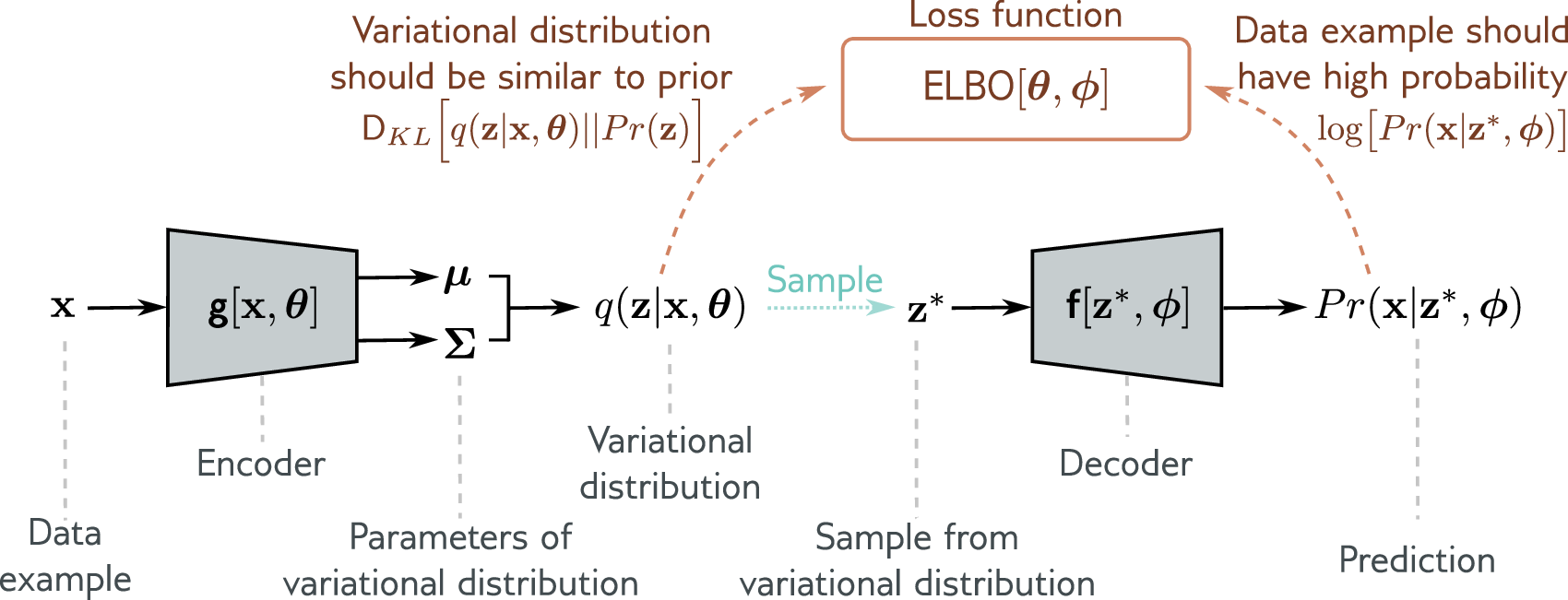
Idea 1: The Decoder
The decoder \(p_\theta(x \mid z)\) is the generator we ultimately want. It is a neural network with parameters \(\theta\) that takes a latent1 vector \(z \in \mathbb{R}^J\) and outputs a probability distribution over protein sequences. At inference time, we sample \(z \sim \mathcal{N}(0, I)\) and decode it into a protein.
class ProteinDecoder(nn.Module):
    """Decodes a latent vector into amino-acid logits for each position."""

    def __init__(self, latent_dim: int, hidden_dim: int, output_dim: int):
        super().__init__()
        self.fc1 = nn.Linear(latent_dim, hidden_dim)
        self.fc2 = nn.Linear(hidden_dim, output_dim)

    def forward(self, z: torch.Tensor):
        h = torch.relu(self.fc1(z))
        return self.fc2(h)  # raw logits; softmax is applied in the loss
For the bead-spring polymer, the decoder is an MLP that maps a 2-dimensional latent vector to 24 output coordinates — three hidden layers of 256 units with ReLU activations. The output is the reconstructed bead positions, not logits: for continuous coordinate data, the decoder directly predicts \(\hat{x} \in \mathbb{R}^{24}\) and the reconstruction loss is mean squared error rather than cross-entropy.
class PolymerDecoder(nn.Module):
    """Decodes a 2D latent vector into 24D polymer coordinates."""

    def __init__(self, latent_dim=2, hidden_dim=256, output_dim=24):
        super().__init__()
        self.net = nn.Sequential(
            nn.Linear(latent_dim, hidden_dim), nn.ReLU(),
            nn.Linear(hidden_dim, hidden_dim), nn.ReLU(),
            nn.Linear(hidden_dim, hidden_dim), nn.ReLU(),
            nn.Linear(hidden_dim, output_dim),
        )

    def forward(self, z):
        return self.net(z)
Idea 2: The Encoder as a Training Trick
In supervised learning, training data comes as (input, label) pairs — the pairing is given. Generative models face a harder problem: there are no pre-assigned latent codes for each training example. The encoder manufactures these pairings.
To train the decoder, we need noise inputs paired with real proteins. The encoder \(q_\phi(z \mid x)\) provides them. Given a training protein \(x\), the encoder infers a distribution over latent vectors that could plausibly map to \(x\):
\[z \sim q_\phi(z \mid x) = \mathcal{N}\!\bigl(\mu_\phi(x),\; \sigma^2_\phi(x) I\bigr)\]Here \(\phi\) denotes the learnable parameters of the encoder, \(\mu_\phi(x) \in \mathbb{R}^J\) and \(\sigma^2_\phi(x) \in \mathbb{R}^J\) are the per-dimension mean and variance, and \(I\) is the \(J \times J\) identity matrix. The distribution \(q_\phi(z \mid x)\) is called the approximate posterior2 because it approximates the true (intractable3) posterior \(p(z \mid x)\).
Training works as follows: for each training protein \(x\), the encoder proposes a distribution over noise inputs \(z\); we sample a \(z\) from that distribution and ask the decoder to reconstruct \(x\) from it. The reconstruction loss trains both networks jointly—the encoder to propose useful noise inputs, the decoder to recover proteins from them.
import torch
import torch.nn as nn

class ProteinEncoder(nn.Module):
    """Encodes a protein sequence into Gaussian parameters (mu, log-variance)."""

    def __init__(self, input_dim: int, hidden_dim: int, latent_dim: int):
        super().__init__()
        self.fc1 = nn.Linear(input_dim, hidden_dim)
        self.fc_mu = nn.Linear(hidden_dim, latent_dim)      # mean of q(z|x)
        self.fc_logvar = nn.Linear(hidden_dim, latent_dim)   # log-variance of q(z|x)

    def forward(self, x: torch.Tensor):
        h = torch.relu(self.fc1(x))
        mu = self.fc_mu(h)
        logvar = self.fc_logvar(h)  # outputting log(sigma^2) keeps sigma > 0
        return mu, logvar
We output \(\log \sigma^2\) rather than \(\sigma^2\) directly. Exponentiating a real number always yields a positive result, so this parameterization guarantees positive variance without needing explicit constraints.
For the polymer, the encoder maps 24D coordinates to a 2-dimensional latent space — the same three-hidden-layer MLP in reverse. An alternative to the log-variance parameterization is the softplus function (\(\log(1 + e^x)\)), which directly outputs a positive standard deviation \(\sigma\). Both guarantee positivity; softplus is smoother near zero.
class PolymerEncoder(nn.Module):
    """Encodes 24D polymer coordinates into 2D Gaussian parameters (mu, sigma)."""

    def __init__(self, input_dim=24, hidden_dim=256, latent_dim=2):
        super().__init__()
        self.net = nn.Sequential(
            nn.Linear(input_dim, hidden_dim), nn.ReLU(),
            nn.Linear(hidden_dim, hidden_dim), nn.ReLU(),
            nn.Linear(hidden_dim, hidden_dim), nn.ReLU(),
        )
        self.fc_mu = nn.Linear(hidden_dim, latent_dim)
        self.fc_sigma = nn.Linear(hidden_dim, latent_dim)

    def forward(self, x):
        h = self.net(x)
        mu = self.fc_mu(h)
        sigma = nn.functional.softplus(self.fc_sigma(h))  # sigma > 0
        return mu, sigma
Idea 3: KL Regularization
Without regularization, a face VAE might memorize each training face in a unique corner of latent space — moving between corners produces garbage rather than smooth interpolation. The KL term prevents this collapse by keeping the latent distribution close to a standard Gaussian.
Reconstruction alone is not enough. If we only minimize reconstruction error, the encoder can map each protein to a tiny, isolated region of latent space—some arbitrary corner far from the origin. Reconstruction would be perfect: the decoder memorizes which corner corresponds to which protein. But at inference we sample \(z \sim \mathcal{N}(0, I)\), and those arbitrary corners are nowhere near the standard normal. The decoder has never seen noise drawn from the regions it will encounter at test time.
The KL divergence term fixes this mismatch:
\[D_{\mathrm{KL}}\!\bigl(q_\phi(z \mid x) \,\|\, \mathcal{N}(0, I)\bigr)\]This penalty forces the encoder’s output distribution for each training protein to stay close to the standard normal. The latent vectors the decoder sees during training then overlap with the distribution it will sample from at inference. The entire latent space becomes populated: sampling \(z \sim \mathcal{N}(0, I)\) and decoding it produces a valid protein, because the decoder has been trained on noise drawn from exactly this region.
The balance between these two terms matters in practice. For continuous coordinate data like the bead-spring polymer, the reconstruction loss (MSE) and KL loss operate on different scales — MSE over 24 coordinates versus KL over 2 latent dimensions. The \(\beta\)-VAE (Higgins et al., 2017) introduces a weighting parameter: \(\mathcal{L} = \text{Reconstruction} + \beta \cdot D_{\mathrm{KL}}\). Setting \(\beta = 0.01\) lets the model first learn faithful coordinate reconstruction before organizing the latent space. With \(\beta = 1\) (the standard VAE), the KL term dominates early in training and can collapse the latent space before the decoder learns anything useful.
To summarize the two loss terms intuitively:
- Reconstruction loss: the decoder should recover \(x\) from the proposed \(z\).
- KL loss: the proposed \(z\) should look like standard normal noise.
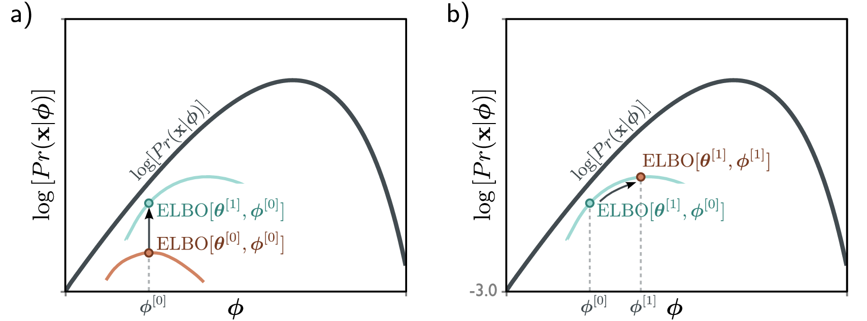
3. The ELBO: Formalizing the Training Objective
Motivation
Section 2 motivated the two loss terms intuitively: reconstruct the data, and keep the encoder’s output close to the prior4. Here we derive these terms from a single principled objective.
Our generative model defines the probability of a protein \(x\) by integrating over all possible noise inputs:
\[p_\theta(x) = \int p_\theta(x \mid z)\, p(z)\, dz\]We want to maximize this marginal likelihood5—the probability that our decoder, fed with random noise from the prior, produces the training proteins. This is exactly the right objective for a generative model: if \(p_\theta(x)\) is high for all training proteins, then sampling \(z \sim \mathcal{N}(0, I)\) and decoding is likely to produce realistic outputs.
The integral is intractable—it sums the decoder’s output over every conceivable \(z\). The encoder \(q_\phi(z \mid x)\) from Section 2 provides the way forward: rather than integrating over all \(z\), we focus on the values of \(z\) that the encoder considers plausible for each \(x\).
Deriving the Evidence Lower Bound
Variational inference sidesteps the intractable integral by deriving a tractable lower bound on \(\log p_\theta(x)\). We introduce the encoder distribution \(q_\phi(z \mid x)\) by multiplying and dividing inside the integral:
\[\log p_\theta(x) = \log \int \frac{p_\theta(x \mid z)\, p(z)}{q_\phi(z \mid x)}\; q_\phi(z \mid x)\, dz\]Recognizing the right-hand side as an expectation6 under \(q_\phi(z \mid x)\), we apply Jensen’s inequality7. Because \(\log\) is a concave function8, we have \(\log \mathbb{E}[Y] \geq \mathbb{E}[\log Y]\) for any random variable \(Y > 0\):
\[\log p_\theta(x) \geq \int q_\phi(z \mid x) \log \frac{p_\theta(x \mid z)\, p(z)}{q_\phi(z \mid x)}\, dz\]Splitting the logarithm of the fraction yields two terms:
\[\underbrace{\int q_\phi(z \mid x) \log p_\theta(x \mid z)\, dz}_{\text{reconstruction term}} \;+\; \underbrace{\int q_\phi(z \mid x) \log \frac{p(z)}{q_\phi(z \mid x)}\, dz}_{\text{negative KL divergence}}\]Recognizing the second integral as the negative Kullback-Leibler (KL) divergence9, we arrive at the Evidence Lower Bound (ELBO):
\[\text{ELBO}(\phi, \theta; x) = \mathbb{E}_{q_\phi(z \mid x)}\!\bigl[\log p_\theta(x \mid z)\bigr] - D_{\mathrm{KL}}\!\bigl(q_\phi(z \mid x) \,\|\, p(z)\bigr)\]The relationship to the marginal log-likelihood is:
\[\log p_\theta(x) \geq \text{ELBO}\]Maximizing the ELBO pushes up on the true log-likelihood from below.
Interpreting the Two Terms
The two terms of the ELBO correspond exactly to the two intuitions from Section 2.
Reconstruction term \(\mathbb{E}_{q_\phi(z \mid x)}[\log p_\theta(x \mid z)]\): sample a latent code \(z\) from the encoder, pass it through the decoder, and measure how well the original protein \(x\) is recovered. Maximizing this term encourages faithful reconstruction. In practice, this is implemented as the negative cross-entropy between the decoder’s output distribution and the true amino-acid sequence.
KL term \(D_{\mathrm{KL}}(q_\phi(z \mid x) \,\|\, p(z))\): this penalizes the encoder for producing distributions that stray too far from the prior \(\mathcal{N}(0, I)\). This is the formal version of the inference-time mismatch argument: without this term, the encoder’s proposed noise values would not overlap with the standard normal we sample from at generation time.
Closed-Form KL for Gaussians
When both \(q_\phi(z \mid x)\) and \(p(z)\) are Gaussian, the KL divergence has a closed-form expression. Let \(q_\phi(z \mid x) = \mathcal{N}(\mu, \mathrm{diag}(\sigma^2))\) with \(\mu \in \mathbb{R}^J\) and \(\sigma \in \mathbb{R}^J\), and let \(p(z) = \mathcal{N}(0, I)\). Then:
\[D_{\mathrm{KL}} = -\frac{1}{2} \sum_{j=1}^{J} \bigl(1 + \log \sigma_j^2 - \mu_j^2 - \sigma_j^2\bigr)\]def kl_divergence(mu: torch.Tensor, logvar: torch.Tensor) -> torch.Tensor:
"""Closed-form KL divergence: KL(N(mu, sigma^2) || N(0, I)).
Args:
mu: encoder mean, shape [batch_size, latent_dim]
logvar: encoder log-variance, shape [batch_size, latent_dim]
Returns:
KL divergence per example, shape [batch_size]
"""
# logvar = log(sigma^2), so exp(logvar) = sigma^2
return -0.5 * torch.sum(1 + logvar - mu.pow(2) - logvar.exp(), dim=-1)
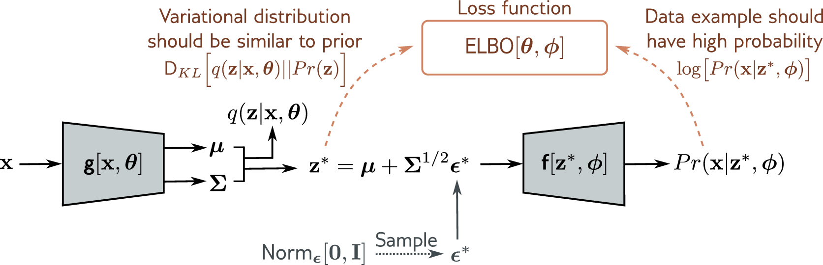
4. The Reparameterization Trick
The Problem
Training the ELBO requires computing gradients of the reconstruction term with respect to the encoder parameters \(\phi\). But this term involves sampling \(z\) from \(q_\phi(z \mid x)\), and sampling is not a differentiable operation. Gradient-based optimizers cannot backpropagate through a random number generator.
The Solution
Kingma and Welling’s reparameterization trick rewrites the sampling step as a deterministic transformation of a fixed noise source. Instead of drawing \(z \sim \mathcal{N}(\mu, \sigma^2 I)\) directly, we draw auxiliary noise \(\epsilon \sim \mathcal{N}(0, I)\), where \(\epsilon \in \mathbb{R}^J\), and compute:
\[z = \mu + \sigma \odot \epsilon\]where \(\odot\) denotes element-wise multiplication. The randomness now resides entirely in \(\epsilon\), which does not depend on any learnable parameter. The mapping from \(\epsilon\) to \(z\) is a deterministic, differentiable function of \(\mu\) and \(\sigma\), so standard backpropagation applies.
Think of it this way: rather than asking “what is the gradient of a coin flip?”, we ask “what is the gradient of a shift-and-scale operation?” The latter is elementary calculus.
def reparameterize(mu: torch.Tensor, logvar: torch.Tensor) -> torch.Tensor:
    """Sample z = mu + sigma * epsilon, where epsilon ~ N(0, I).

    This makes the sampling step differentiable w.r.t. mu and logvar.
    """
    std = torch.exp(0.5 * logvar)   # sigma = exp(log(sigma^2) / 2)
    eps = torch.randn_like(std)      # epsilon ~ N(0, I)
    return mu + eps * std
5. Case Study: Bead-Spring Polymer VAE
Every concept from Sections 1–4 — the decoder, the encoder, KL regularization, the ELBO, the reparameterization trick — comes together in a single working system. The bead-spring polymer introduced in Section 1 provides a concrete testbed: 12 beads in 2D, 24-dimensional coordinate vectors, ~10,000 conformations from molecular dynamics.
Setup and Preprocessing
Raw polymer coordinates contain translation and rotation as nuisance variation. Center-of-mass subtraction removes translation; PCA alignment rotates each conformation so its principal axis aligns with the x-axis. The preprocessed data is flattened to 24-dimensional vectors — the input to the VAE.
def center_com(paths):
    """Subtract center of mass from each conformation."""
    return paths - np.mean(paths, axis=-2, keepdims=True)

def align_principal(paths):
    """Rotate each conformation to align principal axis with x-axis."""
    aligned = np.zeros_like(paths)
    for i, p in enumerate(paths):
        inertia = p.T @ p
        _, evecs = np.linalg.eigh(inertia)
        axis = evecs[:, -1]  # largest eigenvalue
        angle = -np.arctan2(axis[1], axis[0])
        c, s = np.cos(angle), np.sin(angle)
        aligned[i] = p @ np.array([[c, -s], [s, c]]).T
    return aligned

data = align_principal(center_com(paths))
flat_data = data.reshape(-1, 24)  # (N, 24)
The Combined Model
The encoder (24D → 2D latent), reparameterization trick, and decoder (2D → 24D) form a single module. Training minimizes the \(\beta\)-weighted ELBO with \(\beta = 0.01\), MSE reconstruction, and Adam optimization over 150 epochs.
class PolymerVAE(nn.Module):
    def __init__(self, input_dim=24, hidden_dim=256, latent_dim=2):
        super().__init__()
        self.encoder = PolymerEncoder(input_dim, hidden_dim, latent_dim)
        self.decoder = PolymerDecoder(latent_dim, hidden_dim, input_dim)

    def reparameterize(self, mu, sigma):
        eps = torch.randn_like(sigma)
        return mu + sigma * eps

    def forward(self, x):
        mu, sigma = self.encoder(x)
        z = self.reparameterize(mu, sigma)
        x_recon = self.decoder(z)
        return x_recon, mu, sigma
def vae_loss(x, x_recon, mu, sigma, beta=0.01):
    recon = nn.functional.mse_loss(x_recon, x)
    kl = -0.5 * torch.mean(1 + 2 * torch.log(sigma + 1e-8) - mu**2 - sigma**2)
    return recon + beta * kl
Results
After training, the 2D latent space reveals physically meaningful structure. Encoding all training conformations and coloring them by the radius of gyration (\(R_g\) — a measure of how compact or extended the polymer is) produces a smooth gradient across latent space. Compact polymers cluster in one region, extended chains in another — without any \(R_g\) labels during training.
Latent-space interpolation confirms that the space is smooth: linearly interpolating between two latent codes produces a sequence of physically plausible intermediate conformations. Every point along the path decodes to a valid polymer shape.
Property optimization exploits this structure. To find the most compact polymer the model can generate, perform gradient descent on \(R_g\) directly in latent space: start from a random \(z\), compute \(R_g\) of the decoded conformation, backpropagate the gradient to \(z\), and update. After ~200 steps, the optimized polymer is more compact than anything in the training set — the VAE has extrapolated beyond the observed data. This is the same principle behind protein design: encode known proteins, navigate the latent space toward desired properties (binding affinity, stability, solubility), and decode novel sequences.
The full code — data loading, preprocessing, model, training, visualization, and optimization — is in the nano-polymer-vae walkthrough. The companion Lecture 4 applies a diffusion model to the same polymer data, and the nano-polymer-diffusion walkthrough enables a direct side-by-side comparison.
Key Takeaways
Variational autoencoders learn a probabilistic, low-dimensional latent space. The ELBO training objective balances reconstruction fidelity against latent-space regularity (via the KL divergence). The reparameterization trick makes end-to-end training through stochastic sampling possible. Generation is fast—a single decoder pass—and the structured latent space enables interpolation, clustering, and property-guided optimization. The bead-spring polymer case study demonstrates all of these capabilities on a tractable 2D system: a 24-dimensional coordinate space compressed to 2 latent dimensions, with physically meaningful latent structure and gradient-based property optimization.
Further Reading
- Lilian Weng, “From Autoencoder to Beta-VAE” — an accessible walkthrough of variational autoencoders, from vanilla AE to disentangled representations.
- Andrew White, “Variational Autoencoder” — the bead-spring polymer VAE example in JAX, from Deep Learning for Molecules and Materials.
-
The latent code is also called the latent representation, latent variable, or embedding, depending on the community. ↩
-
In Bayesian terminology, the posterior is the distribution over latent variables given observed data. The word “approximate” reminds us that \(q_\phi\) is a parametric family (here, diagonal Gaussians) that may not perfectly match the true posterior. ↩
-
A computation is intractable when it is mathematically well-defined but too expensive to carry out exactly — typically because it requires summing or integrating over an astronomically large space. Tractable is the opposite: the computation has a closed-form solution or an efficient algorithm. ↩
-
In probability, the prior \(p(z)\) is the distribution we assume over latent variables before observing any data. Here the prior is \(\mathcal{N}(0, I)\)—we assume latent codes are standard-normal random vectors. The three Bayesian terms form a chain: the prior \(p(z)\) encodes our initial belief, the likelihood \(p(x \mid z)\) says how probable the data is given a particular \(z\), and the posterior \(p(z \mid x)\) updates the belief after observing data. ↩
-
The likelihood \(p_\theta(x)\) measures the probability the model assigns to observed data. It is called marginal likelihood because we integrate (marginalize) over the latent variable \(z\): \(p_\theta(x) = \int p_\theta(x \mid z)\, p(z)\, dz\). Maximizing it trains the model to consider the training data plausible. ↩
-
The expectation \(\mathbb{E}[Y]\) of a random variable \(Y\) is its average value, weighted by probability. For a continuous variable with density \(p\), it is \(\mathbb{E}[Y] = \int y \, p(y)\, dy\). Think of it as the “center of mass” of the distribution. ↩
-
Jensen’s inequality states that for a concave function \(f\), we have \(f(\mathbb{E}[X]) \geq \mathbb{E}[f(X)]\). Applying it with \(f = \log\) yields the ELBO. ↩
-
A function \(f\) is concave if its graph curves downward — formally, \(f(\lambda a + (1-\lambda) b) \geq \lambda f(a) + (1-\lambda) f(b)\) for any \(\lambda \in [0, 1]\). Convex is the opposite (curves upward, inequality flipped). The logarithm is concave because its slope decreases as its input grows. ↩
-
The KL divergence \(D_{\mathrm{KL}}(q \,\|\, p) = \int q(z) \log \frac{q(z)}{p(z)}\, dz\) measures how different two distributions are. It is always non-negative and equals zero only when \(q = p\). ↩