Transformers for Protein Sequences
This is Lecture 1 of the Protein & Artificial Intelligence course (Spring 2026), co-taught by Prof. Sungsoo Ahn and Prof. Homin Kim at KAIST. It assumes familiarity with the material covered in our preliminary notes on AI fundamentals, protein data and representations, training, and optimization. If any concept feels unfamiliar, please review those notes first.
Introduction
A protein can be 50 residues or 500. A standard linear layer has fixed input and output dimensions—it cannot accept inputs of varying length. Any architecture for proteins must handle variable-length inputs as a first-class concern.
Transformers solve this by letting every residue attend to every other residue, building an input-dependent weight matrix that adapts to any sequence length. They form the architectural backbone of protein language models like ESM-2 and the sequence-processing components of AlphaFold.
This lecture develops transformers from first principles. We begin by asking how neural networks can handle proteins of vastly different lengths, and develop attention as an adaptive linear layer that builds its own weight matrix from the input. We then build the full transformer architecture piece by piece—multi-head attention, feed-forward networks, residual connections, and positional encoding. The companion lecture develops graph neural networks for 3D protein structures.
Roadmap
| Section | Topic | Why it is needed |
|---|---|---|
| 1 | Why attention? | Variable-length inputs and attention as an adaptive linear layer |
| 2 | The attention mechanism | Attention as adaptive weights, the Q/K/V parameterization, scaling, and multi-head attention |
| 3 | The transformer architecture | Attention + FFN + residual connections + normalization, and positional encoding |
1. Why Attention?
A protein can be 50 residues or 500. A standard nn.Linear(in_features, out_features) layer has fixed input and output dimensions—it cannot accept inputs of varying length. Any architecture for proteins must handle variable-length inputs as a first-class concern.
Attention solves this by creating direct connections between every pair of positions. The core idea: attention builds an input-dependent weight matrix—an adaptive linear layer where the same learned parameters produce different behavior for each input. A 50-residue protein produces a \(50 \times 50\) weight matrix; a 500-residue protein produces a \(500 \times 500\) matrix. The same parameters handle both.
2. The Attention Mechanism
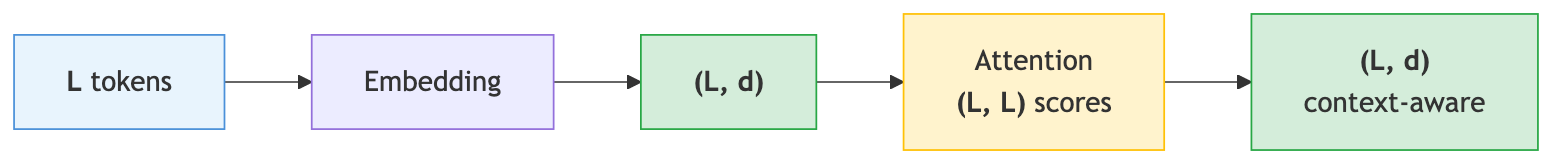
Before diving into the details, here is the big picture of what a transformer does to a protein sequence, traced through the tensor dimensions.
A protein of \(L\) residues starts as a sequence of \(L\) integer tokens. An embedding layer maps each token to a \(d\)-dimensional vector, producing a matrix of shape \((L, d)\) — one row per residue. The attention mechanism computes an \((L, L)\) attention matrix \(A\) that scores every residue-pair relationship, then left-multiplies the embedding: \(AX\) is again \((L, d)\), but now row \(i\) is a weighted combination of all rows of \(X\), with weights determined by \(A_{i,:}\). Each output vector is therefore context-aware — it encodes not just the identity of that residue, but its relationships to all other residues. A transformer block wraps attention with a feed-forward network, residual connections, and normalization, all preserving the \((L, d)\) shape. Stacking \(N\) such blocks produces increasingly refined representations, still \((L, d)\).
In short: the transformer’s input and output have the same shape \((L, d)\). What changes is the meaning of each vector — raw amino-acid identity in, context-aware representation out.
The following sections develop attention from first principles, then assemble it with feed-forward layers, residual connections, and positional encodings into a full transformer.
Attention as Adaptive Weights
A standard linear layer transforms each position independently. Attention’s key insight is to build a weight matrix from the input itself that mixes information across positions. To see why this is necessary, notice the change in how we arrange data compared to the preliminary notes. There, a dataset of \(N\) samples with \(d\) features was stored as \(X \in \mathbb{R}^{N \times d}\), and a linear layer right-multiplied: \(XW\). The rows were independent samples—no interaction between them was needed or desired.
Now the rows of \(X \in \mathbb{R}^{L \times d}\) are positions in a single sequence. To handle a batch of \(N\) sequences simultaneously, we would need a 3-dimensional tensor \(X \in \mathbb{R}^{N \times L \times d}\) and corresponding tensor products in place of matrix multiplications. We ignore the batch dimension throughout this note for notational simplicity—PyTorch handles it automatically. Right-multiplying by \(W \in \mathbb{R}^{d \times d'}\) still gives \(XW \in \mathbb{R}^{L \times d'}\), but each row is transformed independently—there is no cross-position interaction. This is a position-wise linear layer: it can change what each residue’s vector means, but it cannot let residue 50 learn about residue 127.
To mix information across positions, we need to multiply on the other side: left-multiply by a matrix \(A \in \mathbb{R}^{L \times L}\), producing \(AX\). Each row of \(AX\) is now a weighted combination of all input rows—exactly the cross-position interaction we want. But building such an \(A\) is hard: \(A\) must be \(L \times L\), and \(L\) varies from protein to protein. A fixed learned matrix cannot handle this. Simpler alternatives—averaging all position vectors into one, or summing them—do mix information across positions, but they collapse the entire sequence into a single vector, discarding the per-position structure we need.
Attention solves this by computing \(A\) from the input itself. Given a sequence of \(L\) input vectors \(x_1, \dots, x_L \in \mathbb{R}^d\), compute pairwise compatibility scores between all positions, normalize them with softmax, and use the resulting weights to compute weighted averages:
\[\alpha_{ij} = \frac{\exp(x_i^T x_j)}{\sum_k \exp(x_i^T x_k)}, \qquad \text{output}_i = \sum_j \alpha_{ij} \, x_j\]The attention matrix \(A \in \mathbb{R}^{L \times L}\), with entries \(A_{ij} = \alpha_{ij}\), plays the role of the fixed weight matrix \(W\) from a standard linear layer — but \(A\) is computed entirely from the input.
In the sentence “The bank by the river flooded,” the word “bank” should attend strongly to “river” and “flooded” to resolve its meaning—not to “money” or “loan.” A different sentence with the same word would produce entirely different attention weights. The same adaptivity matters for proteins: this is the key insight. Attention is a linear layer whose weight matrix is computed from the data. Fixed layers apply the same transformation to every input; attention builds a different transformation for each input, shaped by the pairwise relationships within it.
Query, Key, Value: Parameterizing Attention
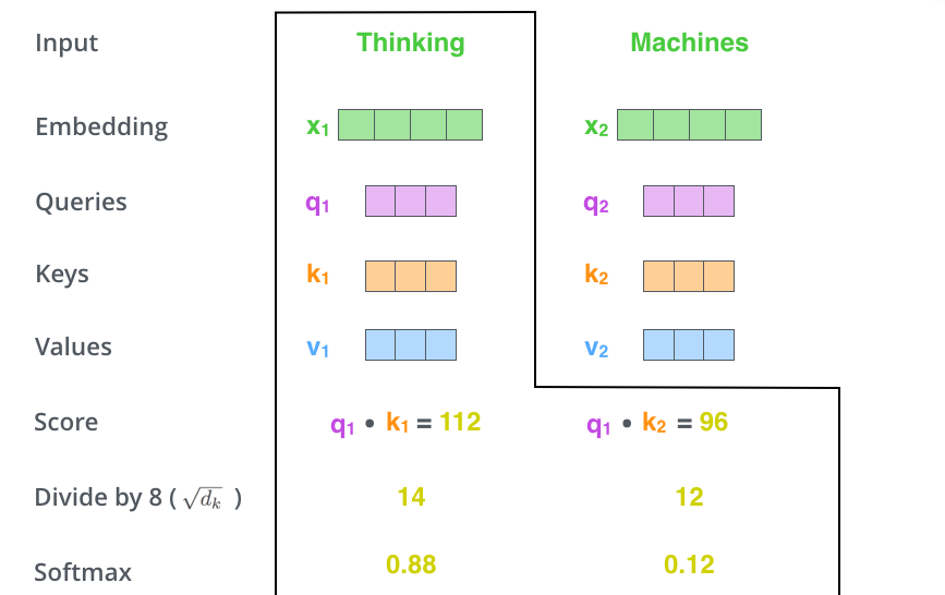
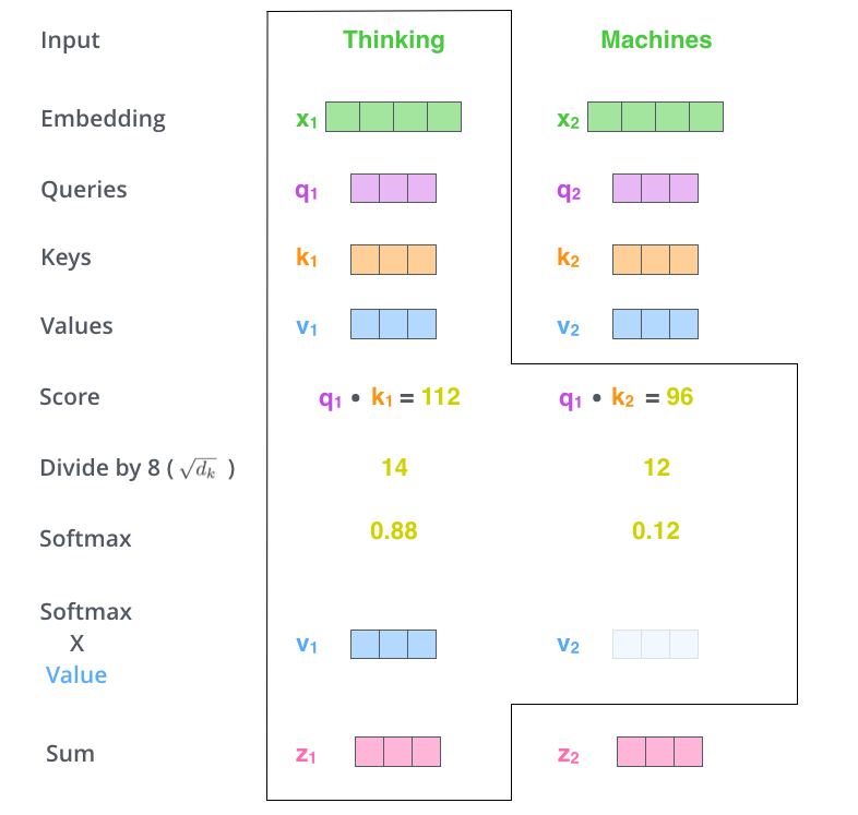
The simple formula \(x_i^T x_j\) uses the same representation for two distinct roles: “what position \(i\) is looking for” and “what position \(j\) has to offer.” Separating these roles with learned linear projections gives the model more flexibility. This is the query-key-value (Q/K/V) decomposition1.
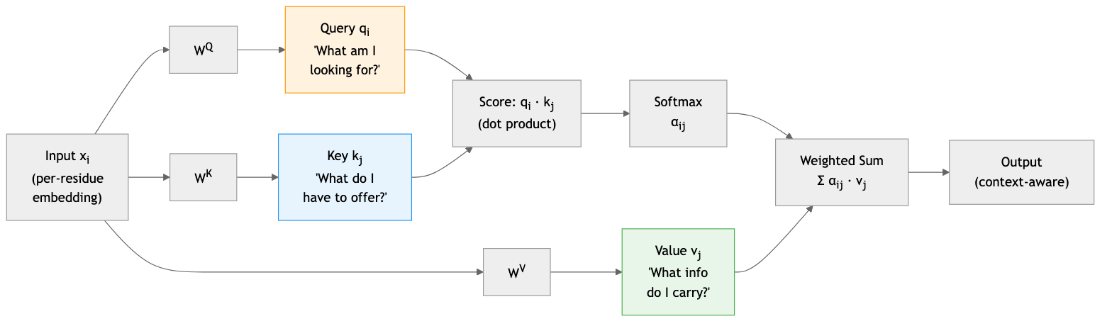
In machine translation, a French word’s query asks “which English words are relevant to my meaning?”, each English word’s key advertises its semantic content, and the value carries the actual information to transfer. In protein sequences, the same decomposition applies: consider a cysteine at position 50 in a protein sequence. Its query \(q_{50}\) encodes what it is looking for—perhaps another cysteine that could form a disulfide bond. The key \(k_{127}\) of a cysteine at position 127 advertises what it has to offer. The value \(v_{127}\) carries the actual information transmitted when position 50 attends to position 127.
Formally, let \(x_i \in \mathbb{R}^d\) be the input representation of position \(i\). We compute the three vectors through learned linear transformations:
\[q_i = W^Q x_i, \qquad k_i = W^K x_i, \qquad v_i = W^V x_i\]Here \(W^Q, W^K \in \mathbb{R}^{d_k \times d}\) and \(W^V \in \mathbb{R}^{d_v \times d}\) are learnable weight matrices, where \(d\) is the input dimension, \(d_k\) is the query/key dimension, and \(d_v\) is the value dimension. The resulting vectors are \(q_i, k_i \in \mathbb{R}^{d_k}\) and \(v_i \in \mathbb{R}^{d_v}\).
The attention score between positions \(i\) and \(j\) is now computed in the projected space:
\[\text{score}_{ij} = q_i \cdot k_j = x_i^T (W^Q)^T W^K x_j\]This dot product measures similarity in the transformed space. If the query and key point in similar directions, the score is high, indicating strong attention. If they point in different directions, the score is low.
We normalize these scores with the softmax function, converting them into a probability distribution:
\[\alpha_{ij} = \frac{\exp(\text{score}_{ij})}{\sum_{k=1}^{N} \exp(\text{score}_{ik})}\]The attention weights \(\alpha_{ij}\) sum to 1 across all positions \(j\). They represent a soft selection: position 50 might attend 40% to position 127, 30% to position 95, 20% to position 143, and distribute the remaining 10% among other positions.
Finally, we compute the output for position \(i\) as a weighted sum of the values:
\[\text{output}_i = \sum_{j=1}^{N} \alpha_{ij} \, v_j\]Positions with high attention weights contribute more. Position 50’s new representation is now informed by its interaction partners, weighted by how relevant each partner is.
Scaled Dot-Product Attention
There is a numerical detail we glossed over above. When the query and key vectors have many dimensions, their dot products can grow large in magnitude. Large scores push the softmax function into regions where its gradients are extremely small2, slowing or stalling training.
The fix is to scale the scores by the square root of the key dimension \(d_k\):
\[\text{Attention}(Q, K, V) = \text{softmax}\!\left(\frac{Q K^T}{\sqrt{d_k}}\right) V\]Here \(Q \in \mathbb{R}^{N \times d_k}\), \(K \in \mathbb{R}^{N \times d_k}\), and \(V \in \mathbb{R}^{N \times d_v}\) are matrices whose rows are the query, key, and value vectors for all \(N\) positions. The scaling factor \(\sqrt{d_k}\) ensures that the variance of the dot products remains approximately 1 regardless of \(d_k\), keeping the softmax in a well-behaved regime.
The following walkthrough traces a single query through all three stages with concrete numbers.
Here is a self-contained implementation:
import torch
import torch.nn as nn
import torch.nn.functional as F
import math


def scaled_dot_product_attention(query, key, value, mask=None):
    """
    Scaled dot-product attention for protein sequences.

    Args:
        query:  (batch, n_heads, seq_len, d_k) — what each residue is looking for
        key:    (batch, n_heads, seq_len, d_k) — what each residue advertises
        value:  (batch, n_heads, seq_len, d_v) — information to transmit
        mask:   optional mask to prevent attention to certain positions
                (e.g., padding tokens in variable-length protein batches)

    Returns:
        output:           (batch, n_heads, seq_len, d_v)
        attention_weights: (batch, n_heads, seq_len, seq_len)
    """
    d_k = query.size(-1)

    # Compute raw attention scores: (batch, n_heads, seq_len, seq_len)
    scores = torch.matmul(query, key.transpose(-2, -1)) / math.sqrt(d_k)

    # Mask out padding positions (set their scores to -inf before softmax)
    if mask is not None:
        scores = scores.masked_fill(mask == 0, float('-inf'))

    # Convert scores to probabilities
    attention_weights = F.softmax(scores, dim=-1)

    # Weighted sum of values
    output = torch.matmul(attention_weights, value)

    return output, attention_weights
Multi-Head Attention
A single set of query, key, and value projections captures one type of pairwise relationship. But real data exhibits many types of relationships simultaneously. In NLP, different heads specialize in different linguistic relationships: one head tracks subject-verb agreement, another resolves pronoun coreference, a third captures semantic similarity between distant words. Proteins are no different. A given residue might need to attend to:
- Nearby positions for local secondary-structure context.
- Distant cysteines for potential disulfide bonds.
- Residues with complementary hydrophobicity for core packing.
- Co-evolving positions that reveal functional constraints.
Multi-head attention runs \(h\) independent attention operations in parallel, each with its own learned projections. Think of each head as a specialist that looks for a specific kind of relationship. Head 1 might learn to identify sequence neighbors. Head 2 might discover potential interaction partners based on amino-acid chemistry. Head 3 might capture secondary-structure patterns. Head 4 might learn functional couplings.
Formally, each head \(i\) computes:
\[\text{head}_i = \text{Attention}(Q W_i^Q,\; K W_i^K,\; V W_i^V)\]where \(W_i^Q \in \mathbb{R}^{d \times d_k}\), \(W_i^K \in \mathbb{R}^{d \times d_k}\), and \(W_i^V \in \mathbb{R}^{d \times d_v}\) are the head-specific projection matrices, and \(d_k = d_v = d / h\).
We concatenate the outputs of all heads and project back to the model dimension with a final weight matrix \(W^O \in \mathbb{R}^{h \cdot d_v \times d}\):
\[\text{MultiHead}(Q, K, V) = \text{Concat}(\text{head}_1, \dots, \text{head}_h)\, W^O\]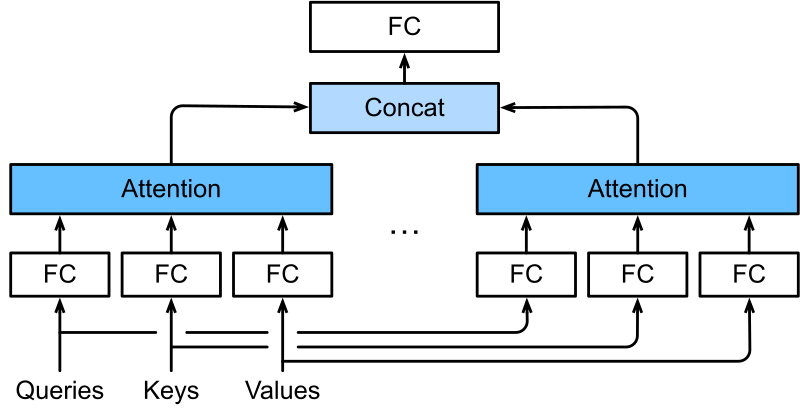
class SelfAttention(nn.Module):
    """
    Multi-head self-attention for protein sequences.

    Each residue attends to all other residues.  Multiple heads
    capture different types of inter-residue relationships.
    """

    def __init__(self, embed_dim, num_heads):
        super().__init__()
        self.embed_dim = embed_dim
        self.num_heads = num_heads
        self.head_dim = embed_dim // num_heads

        # Projection matrices for queries, keys, and values
        self.q_proj = nn.Linear(embed_dim, embed_dim)
        self.k_proj = nn.Linear(embed_dim, embed_dim)
        self.v_proj = nn.Linear(embed_dim, embed_dim)

        # Output projection (applied after concatenating all heads)
        self.out_proj = nn.Linear(embed_dim, embed_dim)

    def forward(self, x, mask=None):
        """
        Args:
            x: (batch, seq_len, embed_dim) — residue embeddings
            mask: optional padding mask

        Returns:
            output: (batch, seq_len, embed_dim) — updated residue embeddings
            attn_weights: (batch, num_heads, seq_len, seq_len)
        """
        batch_size, seq_len, _ = x.shape

        # Compute Q, K, V for all heads simultaneously
        q = self.q_proj(x)  # (batch, seq_len, embed_dim)
        k = self.k_proj(x)
        v = self.v_proj(x)

        # Reshape: split embed_dim into (num_heads, head_dim), then transpose
        q = q.view(batch_size, seq_len, self.num_heads, self.head_dim).transpose(1, 2)
        k = k.view(batch_size, seq_len, self.num_heads, self.head_dim).transpose(1, 2)
        v = v.view(batch_size, seq_len, self.num_heads, self.head_dim).transpose(1, 2)
        # Shape is now: (batch, num_heads, seq_len, head_dim)

        # Scaled dot-product attention
        attn_output, attn_weights = scaled_dot_product_attention(q, k, v, mask)

        # Concatenate heads: transpose back and reshape
        attn_output = attn_output.transpose(1, 2).contiguous().view(
            batch_size, seq_len, self.embed_dim
        )

        # Final linear projection
        output = self.out_proj(attn_output)

        return output, attn_weights
3. The Transformer Architecture

A transformer is more than just attention. It combines several components into a repeating building block called a transformer block. Each block contains four elements:
- Multi-head self-attention — each position attends to all positions, capturing pairwise relationships.
- Layer normalization — normalizes the inputs to each sub-layer, stabilizing training dynamics3.
- Feed-forward network (FFN) — a two-layer MLP applied independently to each position, providing non-linear transformation capacity.
- Residual connections — skip connections that add the input of each sub-layer to its output, facilitating gradient flow and allowing the model to easily preserve information.
The data flow within a single transformer block is:
\[\tilde{x} = \text{LayerNorm}(x + \text{MultiHeadAttention}(x))\] \[x' = \text{LayerNorm}(\tilde{x} + \text{FFN}(\tilde{x}))\]The feed-forward network is typically a two-layer MLP with a wider hidden dimension (often \(4d\)) and a GELU activation:
\[\text{FFN}(x) = W_2 \, \text{GELU}(W_1 x + b_1) + b_2\]where \(W_1 \in \mathbb{R}^{4d \times d}\), \(b_1 \in \mathbb{R}^{4d}\), \(W_2 \in \mathbb{R}^{d \times 4d}\), and \(b_2 \in \mathbb{R}^{d}\).
A complete transformer stacks \(N\) such blocks. Information flows upward through the layers, with each layer refining the residue representations based on increasingly complex patterns.
class TransformerBlock(nn.Module):
    """
    A single transformer block for protein sequence modeling.

    Combines multi-head self-attention with a position-wise
    feed-forward network, using residual connections and
    layer normalization for stable training.
    """

    def __init__(self, embed_dim, num_heads, ff_dim, dropout=0.1):
        super().__init__()

        # Multi-head self-attention sub-layer
        self.attention = nn.MultiheadAttention(
            embed_dim, num_heads, dropout=dropout, batch_first=True
        )
        self.norm1 = nn.LayerNorm(embed_dim)

        # Position-wise feed-forward sub-layer
        self.ff = nn.Sequential(
            nn.Linear(embed_dim, ff_dim),    # Expand to wider hidden dim
            nn.GELU(),                        # Smooth activation function
            nn.Dropout(dropout),
            nn.Linear(ff_dim, embed_dim),     # Project back to model dim
            nn.Dropout(dropout)
        )
        self.norm2 = nn.LayerNorm(embed_dim)

    def forward(self, x, mask=None):
        # Self-attention with residual connection
        attn_out, _ = self.attention(x, x, x, key_padding_mask=mask)
        x = self.norm1(x + attn_out)

        # Feed-forward with residual connection
        ff_out = self.ff(x)
        x = self.norm2(x + ff_out)

        return x
A full protein transformer encoder stacks multiple such blocks:
class TransformerEncoder(nn.Module):
    """
    Transformer encoder for protein sequences.

    Maps a sequence of amino-acid tokens to a sequence of
    context-aware residue embeddings.
    """

    def __init__(self, vocab_size=33, embed_dim=256, num_heads=8,
                 ff_dim=1024, num_layers=6, max_len=1024, dropout=0.1):
        super().__init__()

        # Token embedding: amino acid identity -> vector
        self.token_embed = nn.Embedding(vocab_size, embed_dim)

        # Positional encoding (see next section)
        self.pos_encoding = SinusoidalPositionalEncoding(embed_dim, max_len)

        self.dropout = nn.Dropout(dropout)

        # Stack of transformer blocks
        self.layers = nn.ModuleList([
            TransformerBlock(embed_dim, num_heads, ff_dim, dropout)
            for _ in range(num_layers)
        ])

        self.norm = nn.LayerNorm(embed_dim)

    def forward(self, tokens, mask=None):
        # Embed tokens and add positional information
        x = self.token_embed(tokens)
        x = self.pos_encoding(x)
        x = self.dropout(x)

        # Pass through transformer blocks
        for layer in self.layers:
            x = layer(x, mask)

        return self.norm(x)
Positional Encoding
There is a subtle but important property of the attention mechanism as we have described it: it is permutation-equivariant. If you shuffle the input positions randomly, the outputs are shuffled in the same way. The attention weights depend only on the content of each position, not on where that position sits in the sequence.
“Dog bites man” and “man bites dog” contain identical tokens but have opposite meanings—position determines semantics. This is clearly problematic for proteins as well. Position matters. Two glycines at positions 3 and 4 (consecutive in the backbone) have a very different structural implication than glycines at positions 3 and 300. The backbone connectivity of the chain imposes constraints that depend on sequence position.
The solution is positional encoding: we inject information about each position directly into the input representations.
Sinusoidal positional encoding
The original transformer paper introduced a fixed encoding based on sine and cosine waves at different frequencies. For position \(\text{pos}\) and dimension \(i\):
\[\text{PE}_{(\text{pos},\, 2i)} = \sin\!\left(\frac{\text{pos}}{10000^{2i/d}}\right)\] \[\text{PE}_{(\text{pos},\, 2i+1)} = \cos\!\left(\frac{\text{pos}}{10000^{2i/d}}\right)\]where \(d\) is the embedding dimension. The use of multiple frequencies at different scales allows the model to distinguish both nearby and distant positions. An important property: the encoding of position \(\text{pos} + k\) can be expressed as a linear function of the encoding of position \(\text{pos}\), which means the model can learn to attend to relative positions.
class SinusoidalPositionalEncoding(nn.Module):
    """
    Fixed sinusoidal positional encoding.

    Adds position-dependent patterns to the residue embeddings so that
    the transformer can distinguish position 5 from position 500.
    """

    def __init__(self, embed_dim, max_len=5000):
        super().__init__()

        pe = torch.zeros(max_len, embed_dim)
        position = torch.arange(0, max_len).unsqueeze(1).float()

        # Geometric progression of frequencies
        div_term = torch.exp(
            torch.arange(0, embed_dim, 2).float()
            * (-math.log(10000.0) / embed_dim)
        )

        pe[:, 0::2] = torch.sin(position * div_term)  # Even dimensions
        pe[:, 1::2] = torch.cos(position * div_term)  # Odd dimensions

        # Register as buffer (not a learnable parameter, but saved with model)
        self.register_buffer('pe', pe.unsqueeze(0))

    def forward(self, x):
        # x: (batch, seq_len, embed_dim)
        return x + self.pe[:, :x.size(1)]
Rotary Position Embedding (RoPE)
Modern protein language models such as ESM-2 use Rotary Position Embedding (RoPE)4. Instead of adding positional information to the embeddings, RoPE encodes position through rotations of the query and key vectors. The angle of rotation depends on position, so the dot product between a query at position \(i\) and a key at position \(j\) naturally becomes a function of their relative offset \(i - j\). This elegant approach handles relative positions without the need for explicit relative-position biases.
Key Takeaways
-
Attention enables direct pairwise interactions between all positions in a sequence, handling variable-length inputs through an adaptive weight matrix computed from the input itself.
-
Queries, keys, and values have clear roles: queries ask “what am I looking for?”, keys advertise “what do I have?”, and values carry the information that gets transmitted.
-
Multi-head attention lets the model capture different types of relationships simultaneously—local context, disulfide-bond partners, hydrophobic contacts, co-evolutionary signals—with different heads specializing in different patterns.
-
The transformer architecture combines attention with feed-forward networks, layer normalization, and residual connections into a deep, trainable architecture.
-
Positional encoding is necessary because attention alone has no notion of sequence order.
Further Reading
- Lilian Weng, “Attention? Attention!” — a comprehensive overview of attention mechanisms, from early sequence-to-sequence models to transformers.
- Jay Alammar, “The Illustrated Transformer” — visual step-by-step walkthrough of the Transformer architecture with diagrams.
-
The names query, key, and value come from information retrieval. Think of searching a database: you submit a query, it is matched against keys, and the corresponding values are returned. ↩
-
When one input to softmax is much larger than the others, the output concentrates almost all probability mass on that single element. The gradient with respect to the other elements becomes vanishingly small. ↩
-
Layer normalization computes the mean and variance across the feature dimension for each individual example, in contrast to batch normalization which computes statistics across the batch. Layer normalization is preferred in transformers because it does not depend on batch size. ↩
-
RoPE was introduced by Su et al. (2021) in “RoFormer: Enhanced Transformer with Rotary Position Embedding.” It has since become the default positional encoding in many large language models. ↩