Case Study: Predicting Protein Solubility
This is Preliminary Note 4 for the Protein & Artificial Intelligence course (Spring 2026), co-taught by Prof. Sungsoo Ahn and Prof. Homin Kim at KAIST. It applies everything from Preliminary Notes 1--3 in a complete case study. You should work through this note before the first in-class lecture.
Introduction
Time to build something real. This note is a single, end-to-end project: predicting whether a protein will be soluble when expressed in E. coli, using the solubility dataset from White et al.’s Deep Learning for Molecules and Materials (dmol.pub).
An MLP takes hand-crafted sequence features — amino acid frequencies and physicochemical properties — and outputs a solubility prediction. The architecture is deliberately simple; the interesting problems arise around the model: misleading evaluation, class imbalance, and overfitting. Each section follows the same arc: observe a problem, understand why it happens, introduce a technique that addresses it, show the improvement.
By the end you will have a working solubility predictor and a practical toolkit for diagnosing the most common training problems in protein machine learning. The main lectures introduce more powerful architectures (CNNs, transformers, GNNs) and additional input modalities (3D structure, learned embeddings). A companion code walkthrough builds a convolutional variant of this classifier — learned embeddings and 1D convolutions that exploit sequential structure.
Roadmap
| Section | Topic | What You Will Learn |
|---|---|---|
| 1 | The Solubility Prediction Problem | Why this problem matters and what makes it amenable to ML |
| 2 | The Model: An MLP on Sequence Features | Building a solubility predictor from hand-crafted sequence features |
| 3 | Data Preparation | Dataset/DataLoader setup, train/val/test splitting |
| 4 | Training and Evaluation | Training script, evaluation metrics beyond accuracy, precision-recall |
| 5 | Evaluating Properly: Sequence-Identity Splits | Why random splits overestimate performance, and how to fix it |
| 6 | Handling Class Imbalance | Weighted loss functions for imbalanced datasets |
| 7 | Knowing When to Stop: Early Stopping | Detecting the overfitting point and saving the best model |
| 8 | Debugging and Reproducibility | NaN detection, shape checks, single-batch overfit test, seed setting |
Prerequisites
This note assumes you have worked through Preliminary Notes 1–3: tensors, neural network architectures, loss functions, optimizers, the training loop, data loading, and validation.
1. The Solubility Prediction Problem
Why Solubility Prediction Matters
Expressing recombinant proteins is a core technique in structural biology, biotechnology, and therapeutic development. When a target protein aggregates into inclusion bodies instead of dissolving in the cytoplasm, downstream applications — crystallography, assays, drug formulation — become much harder or impossible. A computational model that predicts solubility from sequence alone can guide construct design and save weeks of experimental effort.
What Makes This Problem Amenable to Machine Learning?
Solubility is influenced by sequence-level properties: amino acid composition, charge distribution, hydrophobicity patterns, and the presence of certain sequence motifs. These patterns are learnable from data. The dataset is a curated collection of 18,453 E. coli proteins from the dmol.pub textbook: each protein is a sequence of amino acids (tokenized as integers 1–20, with 0 for padding), labeled soluble or insoluble. The dataset is roughly balanced — 52% soluble, 48% insoluble.
This is a binary classification task: given a protein sequence, predict whether it will be soluble (1) or insoluble (0). The tools are the same as in Preliminary Note 3: cross-entropy loss, data loading, and the training loop.
2. The Model: An MLP on Sequence Features
Feature Engineering
Rather than feeding raw sequences to the model, the first step is computing a fixed-length feature vector that summarizes each protein’s composition and physicochemical character. This is standard practice for MLP-based protein property prediction: the features encode domain knowledge about what influences solubility.
Each protein produces a 24-dimensional vector:
| Features | Dims | Description |
|---|---|---|
| Amino acid frequencies | 20 | Fraction of each amino acid (A, C, D, …, Y) |
| Sequence length | 1 | Number of residues, normalized |
| Mean hydrophobicity | 1 | Average Kyte-Doolittle score across all residues |
| Net charge | 1 | (K + R + H \(-\) D \(-\) E) / length |
| Fraction charged | 1 | (D + E + K + R) / length |
Amino acid composition is the strongest single predictor of solubility. Insoluble proteins tend to have more hydrophobic residues (I, L, V, F) and fewer charged surface residues (D, E, K, R). The four global descriptors — length, hydrophobicity, charge, and fraction charged — add summary statistics that the MLP can use directly rather than having to reconstruct from the 20 frequencies.
The featurizer compresses a variable-length sequence into a fixed-length vector. This is not optional — an MLP has a fixed number of input neurons, so variable-length sequences must be reduced to a fixed size before the model can process them. Proteins in this dataset range from tens to hundreds of residues; in nature, they span from short peptides (~30 residues) to titin (34,350 residues). Our featurizer handles this by computing aggregate statistics — frequencies, means, ratios — that are well-defined regardless of length. The price: all positional information is lost. A protein with a hydrophobic N-terminus and a charged C-terminus produces the same feature vector as one with the opposite arrangement.
Composition alone is a surprisingly strong baseline for solubility, but the companion code walkthrough shows how convolutional networks can exploit positional patterns for better performance.
The Architecture
import torch
import torch.nn as nn

class SolubilityMLP(nn.Module):
    """
    MLP for predicting protein solubility from hand-crafted features.

    Architecture:
    1. Input: 24-dim feature vector (AA frequencies + physicochemical)
    2. Three hidden layers with ReLU activation and dropout
    3. Linear output: predict soluble (1) vs. insoluble (0)
    """

    def __init__(self, input_dim=24, hidden_dim=128, num_classes=2):
        super().__init__()
        self.net = nn.Sequential(
            nn.Linear(input_dim, hidden_dim),
            nn.ReLU(),
            nn.Dropout(0.3),
            nn.Linear(hidden_dim, hidden_dim),
            nn.ReLU(),
            nn.Dropout(0.3),
            nn.Linear(hidden_dim, 64),
            nn.ReLU(),
            nn.Dropout(0.3),
            nn.Linear(64, num_classes),
        )

    def forward(self, x):
        # x shape: (batch, 24) — feature vector
        return self.net(x)
The model has roughly 28,000 parameters — small enough that it is unlikely to overfit severely on 18,000 training examples, especially with dropout. Compare this to a naive flattened one-hot approach (\(L_{\max} \times 20 = 2{,}000\) input dimensions, ~290,000 parameters): hand-crafted features produce a ten times smaller model because the featurizer compresses the variable-length sequence into a fixed, compact representation before the model sees it.
From Counting to Convolutions
The 20 amino acid frequencies capture composition — what the protein is made of — but not arrangement. A protein with 10% valine scattered evenly looks identical to one with all valines clustered in a single hydrophobic stretch. The clustered version is far more likely to aggregate.
The fix: count not just single amino acids, but pairs of consecutive amino acids (dipeptides). “VV” (two valines in a row) is a different feature from “VD” (valine followed by aspartate). With 20 amino acids, there are \(20^2 = 400\) possible dipeptides:
def dipeptide_frequencies(tokens):
    """Count all 400 dipeptide frequencies."""
    seq = tokens[tokens > 0]
    L = len(seq)
    counts = np.zeros(400)
    for i in range(L - 1):
        pair = (seq[i] - 1) * 20 + (seq[i+1] - 1)
        counts[pair] += 1
    return counts / max(L - 1, 1)
This gives 400 features that capture local context. But why stop at pairs?
| Segment length \(k\) | Features (\(20^k\)) | What it captures |
|---|---|---|
| 1 | 20 | Amino acid composition |
| 2 | 400 | Dipeptide patterns |
| 3 | 8,000 | Tripeptide motifs |
| 4 | 160,000 | Short sequence motifs |
| 5 | 3,200,000 | Approaching full motif-level patterns |
The feature space grows as \(20^k\) — exponential in the segment length. Most of these \(k\)-mers never appear in any protein, so the feature vectors are extremely sparse. With 18,000 training samples and 8,000 features (\(k = 3\)), the model has more dimensions than data points. This is the curse of dimensionality: the feature space grows much faster than the data can fill it.
A 1D convolution solves exactly this problem. A convolutional filter with kernel size \(k\) looks at the same \(k\) consecutive residues as a \(k\)-mer — but instead of enumerating all \(20^k\) possible patterns and counting each one, it learns a small number of useful detectors. A CNN with 16 filters of kernel size 5 replaces 3.2 million possible 5-mer counts with just 16 learned patterns. An embedding layer further compresses each amino acid from a sparse categorical token to a dense vector, so the filter weights are small and the model generalizes well.
The companion code walkthrough builds exactly this: filters of size 5, 3, and 3 in successive layers, each acting as a learned \(k\)-mer detector at increasing effective receptive fields. A 1D CNN is the learned, parameter-efficient generalization of \(k\)-mer frequency counting.
CNNs also handle variable-length input more gracefully than our featurizer: they process each position with the same shared filters, then max-pool the result into a fixed-size vector. No information is lost until the pooling step. But convolutions have their own limitation: locality. A filter of size 5 sees only 5 consecutive residues. Stacking three convolutional layers with pooling gives an effective receptive field of roughly 24 residues — enough for local secondary structure elements, but not for interactions between distant parts of the chain. A disulfide bond between cysteines at positions 30 and 280 is critical for folding and solubility, but no convolutional filter can see both positions at once.
The three approaches compared:
| Approach | Variable length | Positional info | Long-range interactions |
|---|---|---|---|
| Hand-crafted features (this note) | Aggregate to fixed vector | Lost entirely | No |
| 1D CNN (companion walkthrough) | Pad + pool to fixed size | Preserved locally | Limited by receptive field |
| Transformer (Lecture 1) | Native — self-attention over any length | Preserved globally | Every position attends to every other |
Transformers solve both problems at once. Self-attention lets every residue attend to every other residue in a single layer, regardless of distance. The input can be any length — no aggregation, no padding, no fixed receptive field. The cost is quadratic in sequence length (\(O(L^2)\)), but the payoff is capturing long-range dependencies that both hand-crafted features and CNNs miss.
3. Data Preparation
Loading the Dataset
The dmol.pub solubility dataset is a single .npz file containing pre-tokenized protein sequences split into soluble (“positives”) and insoluble (“negatives”). Each sequence is an array of integers: 1–20 for the 20 amino acids, 0 for padding.
import numpy as np
import urllib.request

urllib.request.urlretrieve(
    "https://github.com/whitead/dmol-book/raw/main/data/solubility.npz",
    "solubility.npz",
)
with np.load("solubility.npz") as data:
    pos_data, neg_data = data["positives"], data["negatives"]

print(f"Soluble: {pos_data.shape[0]}, Insoluble: {neg_data.shape[0]}")
print(f"Sequence length (padded): {pos_data.shape[1]}")
# Soluble: 9,667  Insoluble: 8,786  Sequence length: 200
Feature Extraction
Compute the 24-dimensional feature vector for each protein: amino acid frequencies, sequence length, mean hydrophobicity, net charge, and fraction of charged residues.
import torch
from torch.utils.data import TensorDataset, DataLoader
from sklearn.model_selection import train_test_split

features = np.concatenate([pos_data, neg_data], axis=0)
labels = np.concatenate([np.ones(len(pos_data)), np.zeros(len(neg_data))])

# Kyte-Doolittle hydrophobicity scale (alphabetical AA order, matching tokens 1-20)
HYDROPHOBICITY = np.array([
    1.8, 2.5, -3.5, -3.5, 2.8, -0.4, -3.2, 4.5, -3.9, 3.8,   # A C D E F G H I K L
    1.9, -3.5, -1.6, -3.5, -4.5, -0.8, -0.7, 4.2, -0.9, -1.3, # M N P Q R S T V W Y
])

def featurize(tokens):
    """Compute a 24-dim feature vector from an integer-tokenized protein."""
    seq = tokens[tokens > 0]       # remove padding
    L = len(seq)
    if L == 0:
        return np.zeros(24, dtype=np.float32)

    counts = np.bincount(seq, minlength=21)[1:]  # 20 amino acid counts
    freqs = counts / L

    mean_hydro = freqs @ HYDROPHOBICITY

    # Net charge: (K + R + H) - (D + E), per residue
    # Alphabetical 0-indexed: D=2, E=3, H=6, K=8, R=14
    net_charge = (counts[6] + counts[8] + counts[14]
                  - counts[2] - counts[3]) / L

    frac_charged = (counts[2] + counts[3] + counts[8] + counts[14]) / L

    return np.concatenate([
        freqs,             # 20: amino acid composition
        [L / 1000],        #  1: normalized sequence length
        [mean_hydro],      #  1: mean hydrophobicity
        [net_charge],      #  1: net charge per residue
        [frac_charged],    #  1: fraction charged
    ]).astype(np.float32)

X = torch.tensor(np.array([featurize(seq) for seq in features]))  # (N, 24)
y = torch.tensor(labels, dtype=torch.long)
Train / Validation / Test Split
Split with stratification to maintain the class balance in each subset:
X_train, X_test, y_train, y_test = train_test_split(
    X, y, test_size=0.2, stratify=y, random_state=42
)
X_train, X_val, y_train, y_val = train_test_split(
    X_train, y_train, test_size=0.125, stratify=y_train, random_state=42
)

train_loader = DataLoader(TensorDataset(X_train, y_train), batch_size=64, shuffle=True)
val_loader = DataLoader(TensorDataset(X_val, y_val), batch_size=64)
test_loader = DataLoader(TensorDataset(X_test, y_test), batch_size=64)

print(f"Train: {len(X_train)}, Val: {len(X_val)}, Test: {len(X_test)}")
# Train: 12,917  Val: 1,845  Test: 3,691
4. Training and Evaluation
The Training Script
The training pipeline combines per-epoch training with validation monitoring: after each pass through the training data, the model is evaluated on the validation set, and the best-performing checkpoint is saved.
def train_model(model, train_loader, val_loader, epochs=100, lr=1e-3):
    """Full training pipeline with validation monitoring."""
    device = torch.device('cuda' if torch.cuda.is_available() else 'cpu')
    model = model.to(device)

    criterion = nn.CrossEntropyLoss()
    optimizer = torch.optim.AdamW(model.parameters(), lr=lr)

    best_val_loss = float('inf')

    for epoch in range(epochs):
        # --- Training phase ---
        train_loss = train_one_epoch(model, train_loader, criterion, optimizer, device)

        # --- Validation phase ---
        val_loss, _, _ = evaluate(model, val_loader, criterion, device)

        # --- Save best model ---
        if val_loss < best_val_loss:
            best_val_loss = val_loss
            torch.save(model.state_dict(), 'best_model.pt')

        # --- Logging ---
        print(f"Epoch {epoch:3d} | train_loss={train_loss:.4f} | "
              f"val_loss={val_loss:.4f}")

    # Load the best model before returning
    model.load_state_dict(torch.load('best_model.pt'))
    return model

# Instantiate the model and inspect its size
model = SolubilityMLP(input_dim=24, hidden_dim=128, num_classes=2)
n_params = sum(p.numel() for p in model.parameters())
print(f"SolubilityMLP: {n_params:,} parameters")

# Train with validation monitoring
trained_model = train_model(model, train_loader, val_loader, epochs=50)
Evaluation: Beyond Accuracy
Accuracy alone is deceptive. If 70% of proteins are soluble, a model that always predicts “soluble” achieves 70% accuracy while being completely useless.
from sklearn.metrics import (accuracy_score, precision_recall_fscore_support,
                             roc_auc_score)

def evaluate_classifier(model, test_loader, device):
    """Evaluate a binary classifier with multiple metrics."""
    model.eval()
    all_preds = []
    all_labels = []
    all_probs = []

    with torch.no_grad():
        for batch_x, batch_y in test_loader:
            x = batch_x.to(device)
            y = batch_y

            logits = model(x)                               # Raw scores
            probs = F.softmax(logits, dim=-1)               # Probabilities
            preds = logits.argmax(dim=-1)                   # Predicted class

            all_preds.extend(preds.cpu().numpy())
            all_labels.extend(y.numpy())
            all_probs.extend(probs[:, 1].cpu().numpy())     # P(soluble)

    # Compute metrics
    accuracy = accuracy_score(all_labels, all_preds)
    precision, recall, f1, _ = precision_recall_fscore_support(
        all_labels, all_preds, average='binary'
    )
    auc = roc_auc_score(all_labels, all_probs)

    print(f"Accuracy:  {accuracy:.4f}")
    print(f"Precision: {precision:.4f}")
    print(f"Recall:    {recall:.4f}")
    print(f"F1 Score:  {f1:.4f}")
    print(f"AUC-ROC:   {auc:.4f}")

    return accuracy, precision, recall, f1, auc
Understanding the Metrics
All classification metrics are defined in terms of four counts: true positives (TP), false positives (FP), true negatives (TN), and false negatives (FN).
\[\text{Precision} = \frac{TP}{TP + FP}, \qquad \text{Recall} = \frac{TP}{TP + FN}\] \[F_1 = \frac{2 \cdot \text{Precision} \cdot \text{Recall}}{\text{Precision} + \text{Recall}} = \frac{2 \cdot TP}{2 \cdot TP + FP + FN}\]The \(F_1\) score is the harmonic mean of precision and recall — it is high only when both are high.
AUC-ROC (Area Under the Receiver Operating Characteristic curve) plots the true positive rate (recall) against the false positive rate (\(FP / (FP + TN)\)) as the classification threshold varies from 0 to 1, and computes the area under this curve. An AUC of 1.0 means the model achieves perfect separation at some threshold; 0.5 means no better than random.
| Metric | Question It Answers | Protein Example |
|---|---|---|
| Accuracy | What fraction of all predictions are correct? | 85% of solubility predictions correct |
| Precision | Of positive predictions, what fraction truly are? | Of proteins predicted soluble, how many truly are? |
| Recall | Of true positives, what fraction did we detect? | Of truly soluble proteins, how many did we find? |
| F1 Score | Harmonic mean of precision and recall | Balance between missing soluble proteins and wasting experiments |
| AUC-ROC | How well does the model separate classes across all thresholds? | Overall ability to distinguish soluble from insoluble |
The precision-recall tradeoff deserves special attention. In a drug discovery setting, where expressing each candidate is expensive, a biologist might want high precision: “I only want to express proteins that are very likely to be soluble.” By raising the classification threshold from 0.5 to 0.8, we predict fewer proteins as soluble but are more confident in those predictions.
Conversely, in a high-throughput screening setting with thousands of candidates, a biologist might prefer high recall: “I don’t want to miss any potentially soluble protein.” Lowering the threshold to 0.3 captures more true positives at the cost of more false positives.
The AUC-ROC summarizes this tradeoff across all possible thresholds. An AUC of 1.0 means perfect separation; 0.5 means the model is no better than random.
Analyzing the Loss Curves
After training for 50 epochs, examine the loss curves.
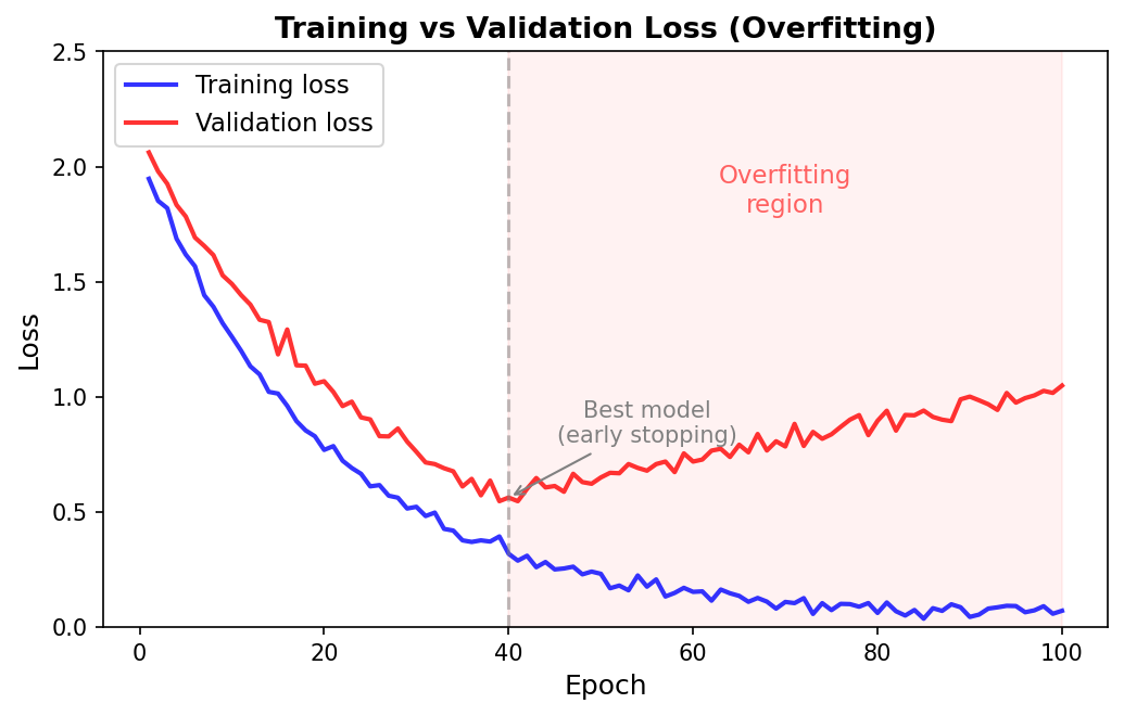
If the training loss decreases smoothly but the validation loss rises after approximately 40 epochs, the model is overfitting. The gap between training accuracy (~98%) and validation accuracy (~72%) confirms this. Sections 6 and 7 address this problem with weighted losses and early stopping.
5. Evaluating Properly: Sequence-Identity Splits
The Problem
The solubility predictor achieves 85% validation accuracy. Impressive? Not necessarily — it depends on how we split the data.
With a random train/validation/test split, there is a high probability that some test proteins are closely related (>90% sequence identity) to proteins in the training set. These homologous proteins almost certainly share the same solubility status. The model can score well by memorizing similar sequences rather than learning true sequence-to-solubility patterns. This is data leakage — the test set contains information that was effectively available during training.
The Solution: Sequence-Identity Splits
The fix relies on sequence clustering: group proteins so that any two proteins in the same group are similar (above some sequence-identity threshold), while proteins in different groups are dissimilar.
A clustering tool like MMseqs2 compares every pair of proteins in the dataset and computes their sequence identity1 — the fraction of aligned positions where the amino acids match.
It then groups proteins into clusters using a threshold (say 30%): if protein A and protein B share \(\geq\) 30% identity, they end up in the same cluster. Each cluster has a representative sequence, and every other member is reachable from the representative through a chain of pairwise alignments above the threshold.
For example, with 10,000 proteins and a 30% identity threshold, you might get 3,000 clusters. Some clusters contain a single unique protein; others contain dozens of close homologs. The crucial property is that proteins in different clusters share less than 30% identity, so they are genuinely different from one another.
The split happens at the cluster level, not the individual protein level: all members of a cluster go into the same split (train, validation, or test). This ensures that no test protein is closely related to any training protein.
import subprocess
import numpy as np

def create_sequence_identity_splits(fasta_file, identity_threshold=0.3, train_ratio=0.8):
    """Split proteins into train/val/test sets respecting sequence identity.

    Requires MMseqs2 to be installed (https://github.com/soedinglab/MMseqs2).
    """
    # Step 1: Cluster proteins at the specified identity threshold
    subprocess.run([
        'mmseqs', 'easy-cluster',
        fasta_file, 'clusters', 'tmp',
        '--min-seq-id', str(identity_threshold)
    ])

    # Step 2: Parse cluster assignments
    clusters = parse_cluster_file('clusters_cluster.tsv')

    # Step 3: Shuffle and split clusters (not individual proteins)
    cluster_ids = list(clusters.keys())
    np.random.shuffle(cluster_ids)

    n_clusters = len(cluster_ids)
    n_train = int(n_clusters * train_ratio)
    n_val = int(n_clusters * 0.1)

    train_clusters = cluster_ids[:n_train]
    val_clusters = cluster_ids[n_train:n_train + n_val]
    test_clusters = cluster_ids[n_train + n_val:]

    # Step 4: Collect protein IDs from the assigned clusters
    train_ids = [pid for c in train_clusters for pid in clusters[c]]
    val_ids = [pid for c in val_clusters for pid in clusters[c]]
    test_ids = [pid for c in test_clusters for pid in clusters[c]]

    return train_ids, val_ids, test_ids
The Reality Check
Retraining with sequence-identity splits instead of random splits, the test accuracy typically drops by 5–15 percentage points. This drop reflects the true difficulty of the task: predicting solubility for proteins that are genuinely different from anything in the training set.
The random-split accuracy was a mirage. The sequence-identity-split accuracy is the honest answer. Any paper that reports performance without controlling for sequence similarity should be read with skepticism.
A word of caution: even 30% sequence identity splits may not be sufficient for all tasks. Proteins from the same CATH2 superfamily can share structural features despite having diverged below 30% identity. For the most rigorous evaluation, consider splitting at the fold or superfamily level.
6. Handling Class Imbalance
The Problem
After switching to sequence-identity splits, a new pattern emerges: the model’s performance on insoluble proteins is much worse than on soluble ones. The dataset after clustering is 70% soluble and only 30% insoluble. The model has learned a shortcut: predicting “soluble” for everything gives 70% accuracy with no effort.
Weighted Loss Functions
The simplest correction: assign higher weights to underrepresented classes, so that misclassifying an insoluble protein incurs a larger penalty:
def compute_class_weights(labels, num_classes):
    """Compute inverse-frequency weights for class-balanced training."""
    counts = torch.bincount(labels.flatten(), minlength=num_classes).float()
    weights = 1.0 / (counts + 1)                    # Inverse frequency
    weights = weights / weights.sum() * num_classes  # Normalize
    return weights

# Apply to our solubility dataset
class_weights = compute_class_weights(train_labels, num_classes=2)
criterion = nn.CrossEntropyLoss(weight=class_weights)
With weighted loss, the model is penalized more heavily for misclassifying the minority class (insoluble proteins). This forces it to pay attention to features that distinguish insoluble proteins rather than defaulting to “soluble.”
Effect on the Model
After applying class weights, the overall accuracy may drop slightly (the model can no longer cheat by always predicting the majority class), but the F1 score and recall for the minority class improve substantially. This is the metric that matters: a model that correctly identifies insoluble proteins is far more useful than one that achieves high accuracy by ignoring them.
7. Knowing When to Stop: Early Stopping
The Problem
Even with regularization (dropout in our model), there comes a point when continued training hurts more than it helps. Validation loss may start rising again after reaching its best value, indicating that the model is beginning to overfit to the training data.
Early Stopping
Early stopping is a form of regularization based on time rather than architecture. The idea: monitor validation performance during training and stop when it stops improving.
Why does this work as regularization? In the early phases of training, the model learns general, transferable patterns. As training continues, it gradually begins to memorize training-specific noise. The point at which validation performance peaks is the sweet spot between underfitting and overfitting.
class EarlyStopping:
    """Stop training when validation loss stops improving."""
    def __init__(self, patience=10, min_delta=1e-4):
        self.patience = patience
        self.min_delta = min_delta
        self.best_loss = float('inf')
        self.counter = 0
        self.should_stop = False

    def step(self, val_loss):
        """Call once per epoch. Returns True if this is a new best model."""
        if val_loss < self.best_loss - self.min_delta:
            self.best_loss = val_loss
            self.counter = 0
            return True   # New best — save checkpoint
        else:
            self.counter += 1
            if self.counter >= self.patience:
                self.should_stop = True
            return False  # No improvement
The training loop checks validation loss after every epoch and saves a checkpoint whenever validation improves. If no improvement occurs for a set number of epochs (the patience), training halts and the best checkpoint is restored.
early_stopping = EarlyStopping(patience=15)

for epoch in range(max_epochs):
    train_loss = train_one_epoch(model, train_loader, criterion, optimizer, device)
    val_loss, _, _ = evaluate(model, val_loader, criterion, device)

    if early_stopping.step(val_loss):
        torch.save(model.state_dict(), 'best_model.pt')

    if early_stopping.should_stop:
        print(f"Early stopping at epoch {epoch}")
        break

# Load the best model for final evaluation
model.load_state_dict(torch.load('best_model.pt'))
EarlyStopping class into the training loop. Each epoch, step() returns True when validation loss improves (save a checkpoint) and sets should_stop = True after patience epochs without improvement.For protein models with small datasets (and therefore noisy validation estimates), a patience of 10 to 20 epochs is typical — long enough to ride out random fluctuations, short enough to avoid wasting computation on a model that has stopped improving.
8. Debugging and Reproducibility
Debugging Neural Networks
Neural networks can fail silently. The code runs, the loss decreases, but predictions are useless. A systematic debugging checklist:
-
Check for NaN gradients — iterate over
model.named_parameters()and checktorch.isnan(param.grad).any(). NaN gradients indicate numerical instability (often from a learning rate that is too large). -
Verify output range — run a forward pass with
torch.no_grad()and printoutput.min()/output.max(). For logits, values should be in a reasonable range (roughly \([-10, 10]\)). -
Check shapes — print input and output shapes at every stage. Shape mismatches (especially after
transposeorunsqueeze) are the most common bug. -
Single-batch overfit test — train on a single batch for 200 steps. If the loss does not approach zero, there is a bug in the architecture, loss function, or data pipeline. This is the single most important debugging technique.
Reproducibility
Set all random seeds (random.seed, np.random.seed, torch.manual_seed, torch.cuda.manual_seed_all) at the start of every experiment. For full GPU determinism, additionally set torch.backends.cudnn.deterministic = True (may slow training by 10–20%).
A Practical Checklist
Before declaring a model “trained,” verify the following:
- Training loss decreases steadily over epochs.
- Validation loss decreases initially, then plateaus (not increases — that signals overfitting).
- The model can perfectly overfit a single batch (sanity check for bugs).
- Gradients are finite (no NaN or Inf values).
- Metrics on the test set are consistent with validation set metrics.
- Results are reproducible when the same seed is used.
Key Takeaways
-
Solubility prediction is a representative binary classification task that exercises every component of the ML pipeline: data preparation, model architecture, training, and evaluation.
-
An MLP on hand-crafted sequence features is a simple but effective starting point. Amino acid composition and physicochemical properties alone carry significant predictive signal for solubility. The main lectures introduce learned representations (embeddings, CNNs, transformers) that extract features directly from raw sequences.
-
Evaluation metrics must go beyond accuracy. Precision, recall, F1, and AUC-ROC tell a more complete story, especially for imbalanced datasets.
-
Sequence-identity splits are mandatory for honest evaluation of protein models. Random splits systematically overestimate performance due to data leakage from homologous sequences.
-
Address class imbalance with weighted losses. High accuracy on an imbalanced dataset is meaningless if the model ignores the minority class.
-
Early stopping saves the best model and prevents wasted computation. Use a patience of 10–20 epochs for protein tasks.
-
Systematic debugging catches silent failures. The single-batch overfit test is the most important sanity check.
-
Sequence identity is reported as a percentage. Rough rules of thumb: above 90% identity, two proteins almost certainly share the same structure and function; above 30–50%, they likely share the same fold; below 20%, the relationship is ambiguous (the “twilight zone” of sequence alignment). ↩
-
CATH is a hierarchical classification of protein domain structures: Class (secondary structure content), Architecture (spatial arrangement), Topology (fold), and Homologous superfamily. ↩