Training Neural Networks for Protein Science
Preliminary Note 3 for the Protein & Artificial Intelligence course (Spring 2026), co-taught by Prof. Sungsoo Ahn and Prof. Homin Kim at KAIST. By the end of this note you will understand every component of the training process—from loss functions through evaluation—and be ready for the solubility case study in Preliminary Note 4.
Introduction
A network fresh off the assembly line knows nothing — its weights are random numbers, and its predictions are meaningless. The loss functions that quantify mistakes, the optimizers that correct them, the training loop that orchestrates the whole process, and the evaluation machinery that tells you whether you have actually learned anything generalizable — these are the subject of this note.
Roadmap
| Section | Topic | Why You Need It |
|---|---|---|
| 1 | Loss Functions | Different prediction tasks require different ways of measuring error |
| 2 | Mini-Batch Training and Optimizers | Why we train on batches, what “stochastic” means, and the algorithms that turn gradients into weight updates |
| 3 | The Training Loop | The four-step cycle that turns data into knowledge |
| 4 | Data Loading for Proteins | Efficient batching, shuffling, and handling of variable-length sequences |
| 5 | Validation, Overfitting, and the Bias-Variance Tradeoff | How to detect when your model is memorizing rather than learning |
Prerequisites
This note assumes familiarity with Preliminary Notes 1 and 2: tensors, nn.Module, activation functions, autograd, gradient descent, and protein features.
1. Loss Functions: Measuring Mistakes
A neural network with random weights outputs meaningless noise. To make it learn, we need a way to quantify how wrong its predictions are, so that gradient descent can push the weights in the right direction.
The loss function (also called a cost function or objective function) does exactly this: a single number measuring prediction quality. Zero means perfect; larger means worse. Every supervised learning task needs a way to measure mistakes. In image classification, the loss quantifies how far the predicted class probabilities are from the true label. In regression tasks like predicting house prices, the loss measures how far the predicted price is from the actual sale price. The same principle applies to proteins: solubility classification needs a different loss than melting temperature regression.
Mean Squared Error (MSE) for Regression
MSE is the standard loss for regression tasks — predicting continuous values. In protein science, this means predicting binding affinity or melting temperature; in a general setting, it means predicting a house’s sale price or a person’s age from a photograph. Let \(y_i\) be the true value and \(\hat{y}_i(\theta)\) be the model’s prediction for example \(i\) (which depends on the current parameters \(\theta\)), with \(n\) examples in total:
\[\mathcal{L}_{\text{MSE}}(\theta) = \frac{1}{n}\sum_{i=1}^{n}(y_i - \hat{y}_i(\theta))^2\]Squaring the error penalizes large mistakes heavily. A prediction that is off by 10 degrees contributes 100 to the sum, while one that is off by 1 degree contributes only 1. This makes \(\mathcal{L}_{\text{MSE}}\) sensitive to outliers — a single wildly mispredicted protein can dominate the loss.
Binary Cross-Entropy (BCE) for Binary Classification
Binary cross-entropy1 appears throughout machine learning: tumor vs. healthy tissue in medical imaging, positive vs. negative sentiment in product reviews, fraudulent vs. legitimate transactions in finance.
BCE is designed for binary classification — tasks with two categories, such as predicting whether a protein is soluble versus insoluble, or whether an email is spam versus not spam. Let \(y_i \in \{0, 1\}\) be the true label and \(\hat{y}_i(\theta) \in (0, 1)\) be the predicted probability:
\[\mathcal{L}_{\text{BCE}}(\theta) = -\frac{1}{n}\sum_{i=1}^{n}\bigl[y_i \log(\hat{y}_i(\theta)) + (1 - y_i)\log(1 - \hat{y}_i(\theta))\bigr]\]Why this formula? It comes from maximum likelihood estimation. If our model predicts \(P(y_i = 1) = \hat{y}_i\), then the probability it assigns to the true label is:
\[P(y_i \mid \mathbf{x}_i; \theta) = \hat{y}_i^{y_i} (1 - \hat{y}_i)^{1 - y_i}\]Assuming training examples are independent, the likelihood2 of the entire dataset is the product \(\prod_i P(y_i \mid \mathbf{x}_i; \theta)\).
Taking the negative log turns this product into a sum (easier to optimize) and flips the sign (so we minimize):
\[-\log \prod_i P(y_i \mid \mathbf{x}_i; \theta) = -\sum_i \bigl[y_i \log \hat{y}_i + (1 - y_i) \log(1 - \hat{y}_i)\bigr] = n \cdot \mathcal{L}_{\text{BCE}}\]So minimizing BCE is equivalent to maximizing the log-likelihood of the data — the model learns to assign high probability to the true labels.
The logarithmic penalty grows without bound as the predicted probability approaches the wrong extreme. When the true label is 1 and we predict \(\hat{y} = 0.99\), the loss is \(-\log(0.99) \approx 0.01\). When we predict \(\hat{y} = 0.01\), the loss is \(-\log(0.01) \approx 4.6\). This creates a strong signal to correct confident mistakes.
Cross-Entropy (CE) for Multi-Class Classification
CE generalizes BCE to multi-class classification — tasks with more than two categories, such as predicting which enzyme class a protein belongs to, or recognizing which of 10 digits appears in a handwritten image. Let \(C\) be the number of classes, \(y_c \in \{0, 1\}\) be the indicator for class \(c\), and \(\hat{y}_c(\theta) \in (0, 1)\) be the predicted probability for class \(c\):
\[\mathcal{L}_{\text{CE}}(\theta) = -\sum_{c=1}^{C} y_c \log(\hat{y}_c(\theta))\]In practice, only one \(y_c\) is 1 (the true class), so this simplifies to \(-\log(\hat{y}_{\text{true class}}(\theta))\). The model is rewarded for assigning high probability to the correct class and penalized (logarithmically) for low probability.
Using Loss Functions in PyTorch
import torch
import torch.nn as nn

# Regression: predict melting temperature
criterion = nn.MSELoss()

# Binary classification: soluble vs. insoluble
# BCEWithLogitsLoss combines sigmoid + BCE for numerical stability
# (your model outputs raw scores, not probabilities)
criterion = nn.BCEWithLogitsLoss()

# Multi-class classification: predict secondary structure (H, E, C)
# CrossEntropyLoss combines softmax + CE for numerical stability
# (your model outputs raw scores, called "logits")
criterion = nn.CrossEntropyLoss()
A practical note: PyTorch’s BCEWithLogitsLoss and CrossEntropyLoss accept logits (raw, unbounded scores) rather than probabilities. They apply sigmoid or softmax internally, which is more numerically stable than applying these functions yourself and then computing the log. This means your model’s output layer should not include a final sigmoid or softmax — let the loss function handle it.
2. Mini-Batch Training and Optimizers
The loss function tells us how wrong we are; the optimizer tells us how to fix it. But first, a more fundamental question: how much data should we use to compute each gradient update?
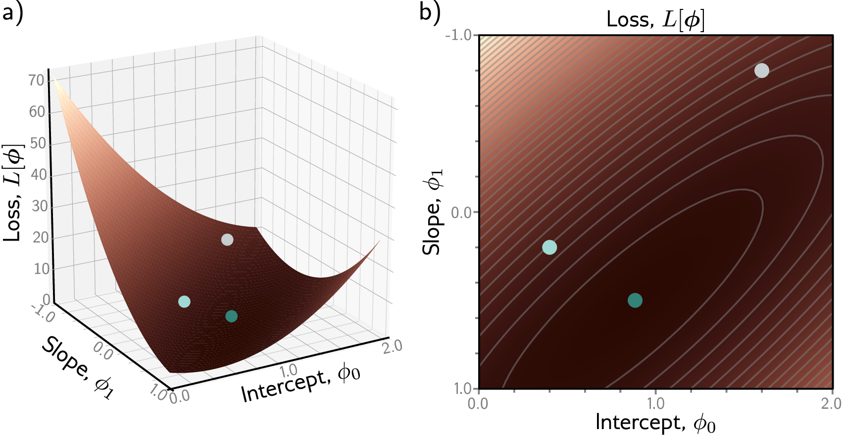
Gradient Descent
The simplest optimizer is (full-batch) gradient descent: compute the loss over the entire training set, then update each weight by taking a step in the direction that reduces it:
\[\theta_{t+1} = \theta_t - \eta \nabla_\theta \mathcal{L}(\theta_t)\]Here \(\theta_t\) represents the current parameter values, \(\eta\) is the learning rate (a small positive number controlling step size), \(\mathcal{L}(\theta_t)\) is the loss function from Section 1 evaluated over all training examples, and \(\nabla_\theta \mathcal{L}(\theta_t)\) is its gradient with respect to the parameters. This is called “full-batch” because the gradient uses every example in the dataset. This is impractical for real datasets — we need the stochastic3 variant.
The learning rate is one of the most important hyperparameters4 in training. Too small, and learning is painfully slow. Too large, and training becomes unstable — the loss oscillates wildly or diverges to infinity.
Mini-Batch Training: Why Not Use All the Data?
ImageNet contains 1.2 million training images — computing the gradient over all of them in a single pass would require hundreds of gigabytes of GPU memory. Mini-batches of 32–256 images make training feasible while providing a noisy but useful gradient estimate. The same logic applies to protein datasets: there is a computational reason and a statistical reason for processing data in small batches rather than all at once.
The computational reason is hardware efficiency. Modern GPUs achieve peak throughput on matrix operations of a specific size — too small and the GPU cores sit idle; too large and the activation tensors overflow GPU memory. A batch of 32–128 proteins hits the sweet spot: large enough for efficient parallelism, small enough to fit in memory. On a typical GPU, a batch matrix multiplication runs hundreds of times faster than processing the same examples one by one in a Python loop5.
The statistical reason is that small random batches provide a noisy but unbiased estimate of the full gradient — and that noise turns out to help generalization (see batch size discussion below).
Suppose your training set contains 50,000 proteins. Full-batch gradient descent processes all 50,000 before taking a single weight update — slow, and the memory required to store all activations simultaneously exceeds any GPU.
Mini-batch stochastic gradient descent is the standard compromise. At each training step, we sample a random subset of \(B\) proteins (the mini-batch) from the training set, compute the average loss over that subset, and update the weights using its gradient:
\[\nabla_\theta \mathcal{L} \approx \frac{1}{B} \sum_{i=1}^{B} \nabla_\theta \ell(\mathbf{x}_i, y_i; \theta)\]Here \(\ell(\mathbf{x}_i, y_i; \theta)\) is the loss for a single example, and \(\mathcal{L}(\theta) = \frac{1}{n}\sum_{i=1}^{n} \ell(\mathbf{x}_i, y_i; \theta)\) is the full-dataset loss. The mini-batch gradient approximates the full gradient using only \(B \ll n\) examples.
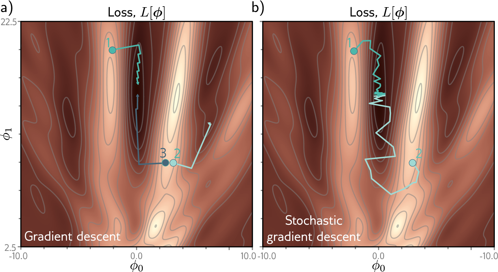
The word stochastic in “stochastic gradient descent” refers to this randomness: at each step, the mini-batch is a random sample, so the gradient is a random variable. The shuffle=True flag in PyTorch’s DataLoader is what makes SGD stochastic — it randomizes which proteins end up in which mini-batch at each epoch.
Batch size controls the noise-accuracy tradeoff. Small batches (16–32) produce noisier gradient estimates, but that noise acts as implicit regularization that helps generalization; they also use less GPU memory. Large batches (256–512) give smoother, more accurate gradients that converge faster per step, but the smoother optimization path can settle into sharp minima that generalize worse. A batch size of 32 or 64 is a reasonable starting point for protein tasks — scale up if GPU memory allows, or drop to 16 if memory is tight.
One epoch means one complete pass through the training set. If the dataset has 50,000 proteins and the batch size is 32, one epoch consists of \(\lceil 50{,}000 / 32 \rceil = 1{,}563\) mini-batch updates. After each epoch, the DataLoader reshuffles the dataset, so mini-batches are different across epochs.
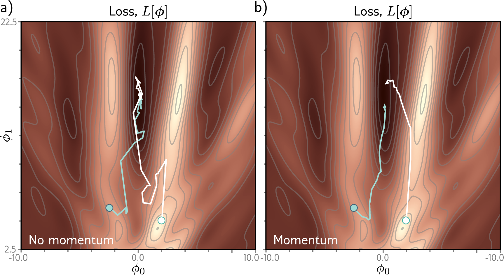
Beyond SGD: Momentum and Adaptive Methods
Vanilla SGD can oscillate when the loss surface curves much more steeply in one direction than another. Momentum fixes this by accumulating a running average of recent gradients, so the optimizer builds speed in consistent directions and dampens oscillations.
Adam [a] goes further by adapting the learning rate individually for each parameter based on its recent gradient history. AdamW [b] is a corrected variant of Adam that handles weight decay properly; it is the recommended default for most protein AI projects.
# AdamW — the recommended default
optimizer = torch.optim.AdamW(model.parameters(), lr=1e-4, weight_decay=0.01)
3. The Training Loop: Four Steps, Repeated
Training is a four-step cycle, repeated once per batch (a subset of examples). One pass through the entire dataset is called an epoch.
Step 1: Forward pass. Feed a batch of proteins through the model to produce predictions. Data flows forward through the network, layer by layer.
Step 2: Compute loss. Compare predictions to true labels using the loss function. This produces a single scalar measuring how wrong we are on this batch.
Step 3: Backward pass. Call loss.backward() to compute gradients for all parameters. Each gradient answers: “how should this weight change to reduce the loss?”
Step 4: Update weights. The optimizer uses the gradients to adjust the weights. We have now learned from this batch.
def train_one_epoch(model, dataloader, criterion, optimizer, device):
    """Train the model for one pass through the dataset."""
    model.train()   # Enable training mode (activates dropout, etc.)
    total_loss = 0

    for batch_x, batch_y in dataloader:
        # Move data to the same device as the model (CPU or GPU)
        batch_x = batch_x.to(device)
        batch_y = batch_y.to(device)

        # Step 1: Forward pass — compute predictions
        predictions = model(batch_x)

        # Step 2: Compute loss — measure prediction error
        loss = criterion(predictions, batch_y)

        # Step 3: Backward pass — compute gradients
        optimizer.zero_grad()   # Clear gradients from the previous batch!
        loss.backward()         # Compute new gradients

        # Optional: clip gradients to prevent exploding values
        torch.nn.utils.clip_grad_norm_(model.parameters(), max_norm=1.0)

        # Step 4: Update weights — apply gradient descent
        optimizer.step()

        total_loss += loss.item()   # .item() extracts a Python float

    avg_loss = total_loss / len(dataloader)
    return avg_loss
A critical detail: optimizer.zero_grad() must be called before each backward pass. By default, PyTorch accumulates gradients — calling .backward() multiple times adds to the existing .grad values rather than replacing them. Without zeroing, gradients from previous batches would contaminate the current update6.
4. Data Loading: Feeding Proteins to Neural Networks
Getting data from disk into the model efficiently is a surprisingly important engineering problem.
The Dataset/DataLoader pattern is universal across deep learning. Image pipelines load JPEGs, resize them to a fixed resolution, and batch them into tensors of shape (batch, C, H, W). NLP pipelines tokenize text, pad sequences to uniform length, and batch them as (batch, seq_len). Protein pipelines follow the same structure: PyTorch separates this into two abstractions: the Dataset (how to access individual examples) and the DataLoader (batching, shuffling, parallel loading).
For our MLP on flattened one-hot sequences, the simplest approach is TensorDataset: pre-encode and pad all sequences, flatten them into feature vectors, wrap the features and labels as tensors, and hand them to a DataLoader.
from torch.utils.data import TensorDataset, DataLoader

# features_flat: shape (N, max_len * 20) — pre-encoded, padded, flattened
# labels: shape (N,) — integer class labels
train_dataset = TensorDataset(features_flat[train_idx], labels[train_idx])
val_dataset = TensorDataset(features_flat[val_idx], labels[val_idx])

# Wrap in DataLoaders
train_loader = DataLoader(
    train_dataset,
    batch_size=32,        # Process 32 proteins at a time
    shuffle=True,         # Randomize order each epoch (important for training)
    num_workers=4,        # Use 4 parallel processes for data loading
    pin_memory=True       # Faster CPU → GPU transfer
)

val_loader = DataLoader(
    val_dataset,
    batch_size=64,        # Larger batches are fine for evaluation (no gradients stored)
    shuffle=False         # Keep a consistent order for reproducible evaluation
)

# Iterate through batches
for batch_x, batch_y in train_loader:
    # batch_x shape: (32, 2000) — flattened one-hot features
    # batch_y shape: (32,) — solubility labels
    pass  # ... feed to model ...
The DataLoader handles three tasks automatically: batching (grouping examples for efficient GPU computation), shuffling (randomizing order each epoch so the model does not learn spurious ordering patterns), and parallel loading (preparing the next batch while the GPU trains on the current one).
The shuffle=True flag is critical — it makes SGD stochastic by randomizing which proteins end up in which mini-batch at each epoch.
5. Validation, Overfitting, and the Bias-Variance Tradeoff
The Bias-Variance Tradeoff
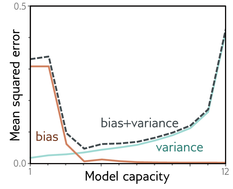
Why not just use the most powerful model available? Because model complexity is a double-edged sword. A linear classifier applied to raw pixels cannot separate cats from dogs — it underfits because the decision boundary is too simple. A 100-million-parameter ResNet trained on only 500 images overfits — it memorizes each training image. The sweet spot lies between these extremes. Bias is the deviation of the model’s average prediction from the true value — averaged over every possible training set we could draw. A linear model predicting solubility from just protein length will systematically miss the real relationship no matter which training proteins it sees. Variance is the spread of the model’s predictions across different training sets drawn from the same distribution. A very complex model fits each training set perfectly, including its noise, so its predictions swing wildly depending on which particular proteins happened to be in the training data. High bias shows up as poor training performance (underfitting); high variance shows up as a large gap between good training performance and poor validation performance (overfitting). The sweet spot is where both metrics are low and close to each other.
The Train/Validation/Test Split
Before training, we divide our data into three non-overlapping subsets, each serving a distinct purpose:
- Training set (~80%): the data the model learns from. The model sees these examples during gradient updates.
- Validation set (~10%): used to monitor generalization during training. We evaluate on this set after each epoch to detect overfitting and to select hyperparameters (learning rate, model size, etc.).
- Test set (~10%): used once, after all training and hyperparameter selection is complete, to report the final performance estimate. This set must never influence any decision during model development.
Why three sets instead of two? If we use the validation set to choose hyperparameters (which we always do), the model’s performance on the validation set is no longer an unbiased estimate of true generalization. We may have inadvertently overfit to the validation set by choosing hyperparameters that happen to work well on it. The test set provides an independent, unbiased estimate.
from sklearn.model_selection import train_test_split

# First split: 80% train, 20% temp
train_df, temp_df = train_test_split(df, test_size=0.2, stratify=df['label'],
                                     random_state=42)

# Second split: 50/50 of temp → 10% validation, 10% test
val_df, test_df = train_test_split(temp_df, test_size=0.5, stratify=temp_df['label'],
                                   random_state=42)

print(f"Train: {len(train_df)}, Val: {len(val_df)}, Test: {len(test_df)}")
Detecting Overfitting
Training loss alone can be misleading. A model might memorize the training examples perfectly (achieving near-zero training loss) without learning patterns that generalize to new proteins. This is overfitting — the central failure mode of machine learning.
The classic signature: training loss decreases steadily, but validation loss starts increasing after some point. The gap between training and validation performance grows over time.
Evaluation follows the same loop as training but with two differences: (1) wrap in torch.no_grad() to skip gradient computation (saving memory and time), and (2) call model.eval() to disable dropout and switch batch normalization to inference mode. After iterating over all batches, compute the average loss and collect predictions for metric computation.
What Overfitting Looks Like
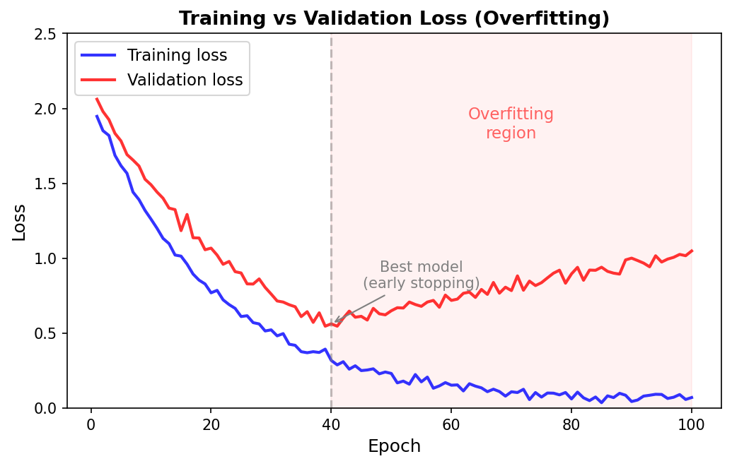
In general, loss curves fall into four patterns:
- Good: both curves decrease and stay close together. The model is learning patterns that generalize.
- Mild overfitting: training loss keeps decreasing, validation loss plateaus. The model has learned what it can but is starting to memorize noise.
- Severe overfitting: training loss approaches zero, validation loss increases. The model is memorizing training data at the expense of generalization.
- Underfitting: both curves are high and flat. The model is too simple to capture the patterns in the data.
Why Protein Models Are Especially Prone to Overfitting
Overfitting is visible in any domain: a medical imaging model achieves 99% training accuracy but only 60% on held-out scans because it memorized scanner-specific artifacts rather than learning disease patterns. Protein datasets are typically small relative to model capacity. A dataset of 5,000 proteins with a model containing 500,000 parameters means there are 100 parameters per training example — plenty of room for the model to memorize each protein individually instead of learning general patterns.
The moment when validation loss stops improving and starts rising is the point of best generalization. Saving the model at that point — and discarding later, overfit versions — is the idea behind early stopping, which we discuss in Preliminary Note 4 alongside other practical techniques for addressing overfitting.
Key Takeaways
-
Loss functions quantify prediction errors. MSE for regression, BCE for binary classification, CE for multi-class. Always use PyTorch’s numerically stable versions (
BCEWithLogitsLoss,CrossEntropyLoss). -
Optimizers turn gradients into weight updates. SGD with momentum is simple and interpretable; AdamW is the recommended default. The learning rate is the single most impactful hyperparameter.
-
Training is a four-step loop — forward pass, loss computation, backward pass, weight update — repeated across many batches and epochs. Don’t forget
optimizer.zero_grad()before each backward pass. -
Data loading with
TensorDatasetandDataLoaderhandles batching, shuffling, and parallel processing. Pre-encode and flatten protein features, then let the DataLoader stream batches to the GPU. -
The bias-variance tradeoff governs model design: too simple models systematically deviate from the truth (high bias), too complex models swing with the training data (high variance). The train/validation/test split is essential for detecting overfitting.
-
Next up: Preliminary Note 4 applies all of these components in a complete case study — predicting protein solubility — including evaluation, sequence-identity splits, class imbalance, and debugging.
References
[a] Kingma, D. P. & Ba, J. (2015). "Adam: A Method for Stochastic Optimization." Proceedings of the 3rd International Conference on Learning Representations (ICLR).
[b] Loshchilov, I. & Hutter, F. (2019). "Decoupled Weight Decay Regularization." Proceedings of ICLR.
-
Entropy measures the average surprise of a random variable — the more unpredictable the outcome, the higher the entropy. Cross-entropy between a true distribution and a predicted distribution measures how surprised the predicted distribution is by the actual outcomes. A perfect predictor has cross-entropy equal to the entropy of the true distribution; any mismatch adds extra cost. ↩
-
The likelihood of a model is the probability it assigns to the observed data. High likelihood means the model considers the data plausible; low likelihood means the model is surprised by it. The log-likelihood is just its logarithm, which turns products into sums and is easier to work with numerically. ↩
-
Stochastic means involving randomness. In stochastic gradient descent, the randomness comes from using a random subset of the data (a mini-batch) to estimate the gradient, rather than computing it exactly over the full dataset. ↩
-
A hyperparameter is a setting chosen by the practitioner before training begins (like learning rate, batch size, or number of layers), as opposed to a parameter learned during training (like the weights of a linear layer). ↩
-
The speedup comes from GPU parallelism: a batch matrix multiplication dispatches all dot products simultaneously across thousands of GPU cores, while a Python loop processes them sequentially with additional interpreter overhead. ↩
-
Gradient accumulation is sometimes used intentionally. When GPU memory is too small for a large batch, you can run several small forward/backward passes, accumulate their gradients, and then call
optimizer.step()once. This simulates training with a larger effective batch size. ↩